Stock Market prediction using Machine Learning

The term stock exchange suggests to a few trades where in portions of openly held organizations are traded. Such money related exercises are directed through conventional trades and by means of over-the-counter (OTC) commercial centres that work under a characterized set of guidelines. Both "stock exchange" and "stock trade" are frequently utilized conversely. Brokers in the financial exchange trade shares on at least one of the stock trades that are essential for the general stock exchange.

The financial exchange permits purchasers and merchants of protections to meet, communicate, and execute. The business sectors take into consideration cost revelation for portions of partnerships and act as an indicator for the general economy. Purchasers and venders are guaranteed of a fair cost, serious level of liquidity, and straightforwardness as market members contend in the open market. The main financial exchange was the London Stock Trade which started in a café, where merchants met to trade shares, in 1773. The principal stock trade in the US started in Philadelphia in 1790. The Buttonwood Understanding, so named in light of the fact that it was endorsed under a buttonwood tree, denoted the start of New York's Money Road in 1792. The understanding was endorsed by 24 merchants and was the principal American association of exchanging stocks kind. The brokers renamed their endeavour the New York Stock and Trade Board in 1817. A stocks exchange is a directed and controlled climate. In the US, the fundamental controllers incorporate the Stocks and Exchange Commission (SEC) and the Financial Industry Regulatory Authority (FINRA).

Libraries used:

NumPy:

NumPy (Numerical Python) is an open-source Python library that is utilized in pretty much every area of science and designing. It is the widespread norm for working with mathematical information in Python, and it is at the core of the logical Python and PyData ecosystems.

Pandas:

Pandas is characterized as an open-source library that gives elite performance data control in Python. The name of Pandas is gotten from the word panel data, and that implies an Econometrics from Complex information. It is utilized for information examination in Python and created by Wes McKinney in 2008.

Matplotlib:

Matplotlib is a thorough library for making static, vivified, and intuitive perceptions in Python. Matplotlib makes simple things simple and hard things conceivable. Make distribution quality plots. Create intelligent figures that can zoom, container, update.

Scikit-learn:

Scikit-learn is an open-source data analysis library, and the best quality level for Machine learning (ML) in the Python ecosystem. Key ideas and elements include: Algorithmic dynamic strategies, including: Order: recognizing and sorting data based of examples.

XG Boost:

This contains the Outrageous Gradient Boosting Machine learning algorithms which is one of the algorithms which assists us with accomplishing high precision on expectations.

Code:

# Here, we will import all this libraries into our program
import numpy as np
import pandas as pd
import matplotlib.pyplot as plt
import seaborn as sb
from sklearn.model_selection import train_test_split
from sklearn.preprocessing import StandardScaler
from sklearn.linear_model import LogisticRegression
from sklearn.svm import SVC
from xgboost import XGBClassifier
from sklearn import metrics
 import warnings
warnings.filterwarnings('ignore')

Importing Dataset:

Any named gathering of records is known as a Dataset. Datasets can hold data, for example, clinical records or protection records, to be utilized by a program running on the framework. Datasets are additionally used to store data required by applications or the working framework itself, for example, source programs, full scale libraries, or framework factors or boundaries. For informational collections that contain discernible text, you can print them or show them on a control center (numerous Datasets contain load modules or other double information that is not exactly printable). Informational collections can be recorded, which allows the Dataset to be alluded to by name without determining where it is put away.

The dataset or CSV file used in this article can be downloaded using this link:

Click Here

# Here, we are reading all the data of the CSV file
ds = pd.read_csv('/content/Tsla.csv')
ds.head()

Output:

Date             Open               High                   Low                  Close          Adj             Volume
         Opening         Highest              Lowest	            Closing      		   Trading
          price	        price                  price	            price			   volume
                                that day            that day
2010-07-07     16.4000            16.629999           14.980000          15.8000         15.8000              6921700
2010-07-08     16.1399            17.520000           15.570000          17.4599         17.4599              7711400
2010-07-09     17.5800            17.900000           16.549999          17.4000         17.4000             4050600
2010-07-12     17.9500            18.070000           17.000000          17.0499         17.0499             2202500
2010-07-13     17.3899            18.639999           16.900000          18.1399         18.1399            2680100

This are the five rows of the CSV file. we can see that data for a portion of the dates is feeling the loss of the reason behind that is on ends of the week and occasions stock market stays closed hence no exchanging occurs on these days.

# Here, we are getting the no. of column and no. of rows of the dataset
ds.shape

Output:

(1705, 7)

From the above output we can clearly say that the total no. of columns available are 7 and the total no. of rows available are 1705 in the dataset or CSV file.

# Here, we are describing our dataset
ds.describe()

Output:

                      Open               High                   Low                  Close          Adj             Volume
         Opening         Highest              Lowest	            Closing      		   Trading
          price	        price                  price	            price			   volume
                                that day            that day
count        1705.0000         1705.0000           1705.0000          1705.000            1705.000         1.7050e+03
mean       130.13992          132.520000         128.57000          130.4599           133.4599          4.2707e+06    
std            94.58002            95.900000           92.549999          94.4000             95.4000            4.2707e+06
min          16.9500             16.070000           14.000000          15.04990           15.0499            1.1850e+05
25%         30.3899             30.639999           29.900000          29.13995             29.10399        1.19435e+06
50%         156.5453            162.45450          153.45645          158.48455          159.54548       3.1807e+04
75%         224.5464            220.56545          215.56545          225.54565          222.56445       5.6621e+09
Max         285.54556          290.55455          280.54545          286.56545          286.56545       3.1763e+02

Exploratory Data Analysis:

EDA is a way to deal with dissecting the information utilizing visual strategies. It is utilized to find patterns, and examples, or to really look at suspicions with the assistance of factual rundowns and graphical portrayals. While playing out the EDA of the Tesla Stock Cost information we will dissect how costs of the stock have moved over the timeframe and what the finish of the quarters means for the costs of the stock.

Example: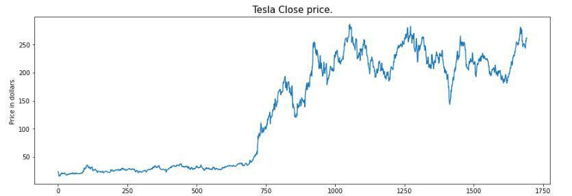

plt.figure(figsize= (18,5))       # here, we are declaring the dimensions of graph
plt.plot(ds['Close'])       
# here, we are giving the title to the graph
plt.title('Tesla Close price.', fontsize=15)
plt.ylabel('Price in dollars.')        # here, we are labelling the y axis
plt.show()          # here, we are showing the graph plotted

Output:

Stock Market prediction using Machine Learning

From the above graph we can see that the tesla stocks are showing an upward trend as shown in the graph.

# Here, we are reading all the data of the CSV file
ds.head()

Output:

Date             Open               High                   Low                  Close          Adj             Volume
         Opening         Highest              Lowest	            Closing      		   Trading
          price	        price                  price	            price			   volume
                                that day            that day
2010-07-07     16.4000            16.629999           14.980000          15.8000         15.8000              6921700
2010-07-08     16.1399            17.520000           15.570000          17.4599         17.4599              7711400
2010-07-09     17.5800            17.900000           16.549999          17.4000         17.4000             4050600
2010-07-12     17.9500            18.070000           17.000000          17.0499         17.0499             2202500
2010-07-13     17.3899            18.639999           16.900000          18.1399         18.1399            2680100

In the output of ds.head(), if we notice cautiously we can see that the information in the 'close' column and that accessible in the 'Adj Close' segment is a similar we should check regardless of whether this is the situation with each column.

Feature Engineering:

Feature engineering helps with getting a few important features from the current ones. These additional features some of the time help in expanding the exhibition of the model altogether and absolutely help to acquire further bits of knowledge into the data.

# here, we are splitting the day, month and the year
splitted = ds['Date'].str.split('/', expand=True)
ds['day'] = splitted[1].astype('int')
ds['month'] = splitted[0].astype('int')
ds['year'] = splitted[2].astype('int')
ds.head()

Output:

Date      Open             High           Low     Close           Adj    Volume       day    month   year
 Opening        Highest      Lowest    Closing      	 Trading
  price	             price           price	     price	volume
                            that day    that day
2010-07-07     16.40            16.62           14.98          15.80         15.80              69217     7       7          2010
2010-07-08     16.13            17.52           15.57          17.45         17.45              77114      8       7         2010
2010-07-09     17.58            17.90           16.54          17.40         17.40             40506        9       7        2010
2010-07-12     17.95            18.07           17.00          17.04         17.04             22025        12      7        2010
2010-07-13     17.38            18.63           16.90          18.13         18.13            26801         13       7        2010

Here, we have splitted the date column into three more columns has day, month, and the year this are already initialized in the date columns previously.

# here, we are checking for the quarter in the given month
ds['quarter'] = np.where(ds['month']%3==0,1,0)
ds.head()

Output:

Date      Open      High         Low     Close           Adj    Volume  Day  month  year  Quarter
          Opening  Highest      Lowest    Closing      	 Trading
  price	       price           price	     price	volume
                   that day    that day
2010-07-07     16.40     16.62      14.98    15.80   15.80    69217     7       7          2010                           0
2010-07-08     16.13      17.52     15.57     17.45    17.45   77114      8       7         2010	             0
2010-07-09     17.58       17.90    16.54     17.40    17.40    40506        9       7        2010                         0
2010-07-12     17.95       18.07     17.00    17.04    17.04    22025        12      7        2010                        0
2010-07-13     17.38       18.63      16.90   18.13    18.13    26801         13       7        2010                      0

A group of three months is called as a quarter. Each organization prepares its quarterly results and distributes them publicly so, that individuals can analyse the organization's performance. These quarterly outcomes influence the stock costs vigorously which is the reason we have added this element since this can be a useful feature for the learning model.

# here, we 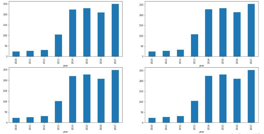are plotting the bar graph for open, high, low and close columns and          # grouping using year
dt_grouped = ds.groupby('year').mean()
plt.subplots(figsize=(25,15))
for i, col in enumerate(['Open', 'High', 'Low', 'Close']):
  plt.subplot(2,2,i+1)
  dt_grouped[col].plot.bar()
plt.show()       # here, we are showing the plotted graph

Output:

By analysing the above bar graph, we can say that the stocks of the tesla have increased twice in the span of year 2013 to the year 2014.

Here are a portion of the important observations of the above-grouped data:

Costs are higher in the months which are quarter end when contrasted with that of the non-quarter end months.
The volume of exchanges is lower in the months which are quarter end.

# Here, we are adding some columns to the program
ds['open-close']  = ds['Open'] - ds['Close']
ds['low-high']  = ds['Low'] - ds['High']
ds['target'] = np.where(ds['Close'].shift(-1) > ds['Close'], 1, 0)

Above we have added a few additional columns which will help in the training of our model. We have added the objective component which is a sign regardless of whether to purchase we will prepare our model to just foresee this. In any case, prior to continuing we should check regardless of whether the objective is adjusted utilizing a pie graph.

# Here, we 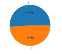are plotting a pie chart for the dataset
plt.pie(ds['target'].value_counts().values,
        labels=[0, 1], autopct='%1.1f%%')
plt.show()

Output:

At the point when we add features to our dataset we need to guarantee that there are no exceptionally related features as they don't help in that learning process with handling of the calculation.

plt.fig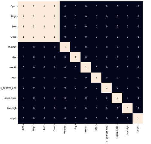ure(figsize=(10, 10))
# As our concern is with the exceptionally
# corresponded includes just thus, we will picture
# our heatmap according to that standards as it were.
sb.heatmap(ds.corr() > 0.9, annot=True, cbar=False)
plt.show()

Output:

From the above heatmap, we can express that there is a high relationship between OHLC that is really obvious, and the additional features are not profoundly connected with one another or recently gave highlights which implies that we are all set and build our model.

Data Splitting and Normalization:

features = ds[['open-close', 'low-high', 'quarter']]
target = ds['target']
scaler = StandardScaler()
features = scaler.fit_transform(features)
X_tra, X_val, Y_tra, Y_val = tra_ts_split(
    features, target, ts_size=0.1, random_state=2022)
print(X_tra.shape, X_val.shape)

Output:

(1435, 3) (190, 3)

After choosing the elements to prepare the model on we should standardize the data in light of the fact that standardized information prompts steady and quick preparation of the model. After that entire information has been parted into two sections with a 90/10 ratio in this way, that we can assess the presentation of our model on concealed data.

Model Development and Evaluation:

This is the ideal opportunity to prepare some cutting edge AI models(Logistic Relapse, Backing Vector Machine, XGB Classifier), and afterward founded on their exhibition on the preparation and approval information we will pick which ML model is filling the need within hand better.

For the assessment metric, we will utilize the ROC-AUC bend however why this is on the grounds that as opposed to anticipating the hard likelihood that is 0 or 1 we would like it to anticipate delicate probabilities that are ceaseless qualities between 0 to 1. Furthermore, with delicate probabilities, the ROC-AUC bend is for the most part used to gauge the precision of the expectations.

Code:

# Here, we are getting the training accuracy and validation accuracy
models = [LogisticRegression(), SVC(
  kernel='poly', probability=True), XGBClassifier()]
for i in range(3):
  models[i].fit(X_tra, Y_tra)
  print(f'{models[i]} : ')
  print('The Training Accuracy of the model is: ', metrics.roc_auc_score(
    Y_tra, models[i].predict_proba(X_tra)[:,1]))
  print('The Validation Accuracy of the model is: ', metrics.roc_auc_score(
    Y_val, models[i].predict_proba(X_val)[:,1]))
  print()

Output:

Logistic Regression():
The Training Accuracy of the model is: 0.5148967
The Validation Accuracy of the model is: 0.5468975

SVC(kernel = ?poly?, probability = True):
The Training Accuracy of the model is: 0.47108955
The Validation Accuracy of the model is: 0.4458765

XGB classifier():
The Training Accuracy of the model is: 0.7856421
The Validation Accuracy of the model is: 0.58462215

Among the three models, we have prepared XGB Classifier has the best presentation but it is pruned to overfitting as the contrast between the preparation and the approval precision is excessively high.

# Here, we 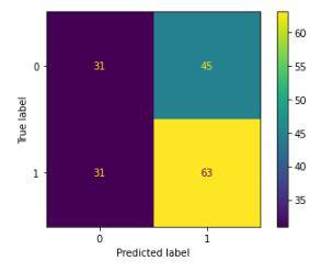are plotting the confusion matrix to the validation data
metrics.plot_confusion_matrix(models[0], X_val, Y_val)
plt.show()

Output:

Confusion matrix

Conclusion:

We can see that the accuracy accomplished by the state-of-the-art ML model is no more excellent than basically speculating with a likelihood of half. Potential purposes behind this might be the absence of information or utilizing an exceptionally basic model to perform such a complex task as Stock Market prediction.

Next TopicHow to Check the Accuracy of your Machine Learning Model

← prev next →