Implementation of neural network from scratch using NumPy

Introduction to Neural Networks:

In the consistently developing scene of artificial knowledge (simulated intelligence), one idea has endured for the long haul and shown to be a foundation of present-day machine learning: artificial neural networks (ANNs). These computational models, propelled by the human mind's unpredictable network of neurons, have shown astounding ability in assignments going from image recognition to natural language handling. In this article, we leave on an excursion to demystify the internal functions of ANNs, with a specific spotlight on why carrying out a neural network from scratch can be a priceless learning experience.

Artificial Neural Networks

Artificial neural networks, frequently called neural networks, have a rich history dating back to the mid-twentieth century. Their origin was propelled by the craving to make machines that could emulate the intricate dynamic cycles of the human cerebrum. Early trailblazers, similar to Plain Rosenblatt and Warren McCulloch, laid the hypothetical preparation for neural networks, while it was only after the appearance of present-day processing that these ideas could be executed for all intents and purposes.

At its center, an artificial neural network is a computational model containing interconnected hubs or neurons. These neurons work cooperatively to process and change input information, at last delivering a result. Every association between neurons is related to a weight, which decides the strength of the association. The neuron applies an initiation capability to the weighted amount of its bits of feedback, acquainting non-linearity with the model.

You could ask why anybody would need to execute a neural network from scratch when strong deep learning libraries like TensorFlow and PyTorch are accessible.
Deep learning structures give pre-assembled neural network layers and preparing techniques, causing complex undertakings to appear to be misleading basic. Even so, this accommodation frequently comes at the expense of understanding.
Building a neural network from scratch considers fine-grained command over each part of the model. At the point when you experience blunders or unforeseen ways of behaving, you won't be left in obscurity.
The field of deep learning is in an unending condition of headway. New models, actuation capabilities, and improvement strategies arise consistently.

Neurons: The Computational Units

At the core of any neural network are neurons. These are the computational units liable for processing data. Neurons get inputs, perform estimations, and produce a result. In a neural network, neurons are coordinated into layers, regularly including an info layer, at least one secret layer, and a result layer. The associations between neurons, each related to weight, empower the data stream.

The Feedforward Process

The feedforward process is the component of information moving through a neural network from the info layer to the result layer. It very well may be summed up as follows:

Input Layer: The information is taken care of in the info layer.

Weighted Total: Every neuron in the ensuing layers works out a weighted amount of its bits of feedback.

Activation Function: The weighted total is gone through an activation function, presenting non-linearity.

Result: The result of the activation function becomes the contribution for the following layer, and the process rehashes until we arrive at the result layer.

Activation Functions: Adding Non-Linearity

Activation functions assume an urgent part in neural networks. They present non-linearity, empowering neural networks to learn complex examples. Two normal activation functions are the sigmoid function and the Corrected Direct Unit (ReLU) function:

Sigmoid Function: It squashes the information values somewhere between 0 and 1, which can be deciphered as probabilities. It's helpful in the result layer of paired characterization issues.

ReLU Function: It yields the information esteem on the off chance it's certain and zero. ReLU has become the default decision for most stowed-away layers because of its effortlessness and viability.

Weight Initialization and Bias Terms

The loads in a neural network are urgent for learning. Weight statement includes setting the underlying upsides of these loads. Normal procedures incorporate an arbitrary introduction, Xavier/Glorot, and He statements. Appropriate weight introduction can altogether influence the preparation process.

Bias terms are added substance constants in neurons. They permit neurons to display more complicated functions by moving the result of the activation function. Every neuron has its bias term.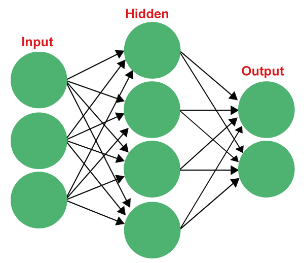

Implementation of neural network from scratch using NumPy

Neural Networks using NumPy

Step 1: Make a Dataset

To work with our neural network, we want a dataset to train and test its exhibition:

Producing Examples: We characterize matrix examples for letters A, B, and C. These examples act as the input data for training and testing the neural network. Each example is a double succession that addresses the state of the separate letter.

Code

# Create a dataset
letter_a = np.array([0, 0, 1, 1, 0, 0, 0, 1, 0, 0, 1, 0, 1, 1, 1, 1, 1, 1, 1, 0, 0, 0, 0, 1, 0, 0, 0, 0, 1])
letter_b = np.array([0, 1, 1, 1, 1, 0, 0, 1, 0, 0, 1, 0, 0, 1, 1, 1, 1, 1, 1, 0, 0, 0, 0, 1, 0, 0, 0, 0, 1])
letter_c = np.array([0, 1, 1, 1, 1, 0, 0, 1, 0, 0, 0, 0, 0, 1, 0, 0, 0, 0, 1, 0, 0, 0, 0, 1, 0, 0, 0, 0, 1])

# Combine the patterns into a dataset
x = np.array([letter_a, letter_b, letter_c])

Step 2: Characterize Labels

For directed learning, we want marks to demonstrate the right responses:

Naming Data: We indicate one-hot encoded marks for the letters A, B, and C. One-hot encoding is a method for addressing downright data mathematically, where every class compares to a remarkable parallel worth. During training, these names permit the neural network to learn and connect designs with their related letters.

Code

# Define labels (one-hot encoding)
y = np. array([[1, 0, 0], [0, 1, 0], [0, 0, 1]])

Step 3: Import Libraries and Characterize Activation Function

In this underlying step, we set up the establishment for our neural network:

Importing Libraries: We import fundamental libraries, like NumPy, for proficient mathematical tasks and Matplotlib for data visualization. These libraries give us the tools we want to build and assess the neural network.

Defining the Sigmoid Activation Function: We characterize the sigmoid activation function, a pivotal part of the neural network. The sigmoid function takes an input and guides it to a worth somewhere between 0 and 1. This function brings non-linearity into the network's output, empowering it to demonstrate complex connections in the data.

Code

import numpy as np
import matplotlib.pyplot as plt

# Activation function (Sigmoid)
def sigmoid(x):
    return 1 / (1 + np.exp(-x))

Step 4: Initialize Weights

In this step, we set up the underlying conditions for the neural network's learnable boundaries:

Weights: We make a function that creates irregular weights for the associations between neurons in the neural network. These weights are fundamental since they control how data courses through the network during training. Introducing them haphazardly permits the network to gain from data and adjust its weights over the long haul.

Code

# Initialize weights randomly
def generate_weights(input_size, output_size):
    return np.random.randn(input_size, output_size)

Step 5: Characterize the Feedforward Neural Network

This step characterizes the engineering and forward pass of our neural network:

Defining the Neural Network Design: We determine the construction of the neural network, remembering the number of layers and neurons for each layer. For this situation, we have an input layer, a hidden layer, and an output layer. The feed_forward function takes an input and figures the network's output by engendering it through these layers.

Code

# Create the Feedforward Neural Network
# Input layer (1, 30)
# Hidden layer (1, 5)
# Output layer (3, 3)
def feed_forward(x, w1, w2):
    # Hidden layer
    z1 = x.dot(w1)  # Input from layer 1
    a1 = sigmoid(z1)  # Output of layer 2

    # Output layer
    z2 = a1.dot(w2)  # Input of output layer
    a2 = sigmoid(z2)  # Output of output layer
    return a2

Step 6: Characterize the Loss Function

In this step, we lay out how the neural network evaluates its presentation:

Defining the Loss Function: We characterize the mean squared error (MSE) loss function, which estimates the distinction between the anticipated output and the genuine objective qualities. The MSE evaluates how well the neural network's predictions align with the genuine data, offering a mathematical benefit the network plans to limit during training.

Code

# Mean Square Error (MSE) Loss Function
def loss(output, target):
    squared_error = np.square(output - target)
    mean_squared_error = np.mean(squared_error)
    return mean_squared_error

Step 7: Backpropagation of Error

In this step, we set up the component for refreshing the neural network's weights in light of prediction errors:

Executing Backpropagation: We carry out the backpropagation calculation, a vital part of training neural networks. Backpropagation computes the slopes of the loss concerning the network's weights, permitting us to change the weights toward a path that lessens the loss. This iterative cycle is essential for the network to learn and work on its presentation.

These essential steps lay the foundation for building, training, and assessing a neural network for different undertakings. The resulting steps in the code expand upon these standards to make a total neural network and apply it to a particular issue.

Code

# Backpropagation of error
def back_propagation(x, y, w1, w2, learning_rate):
    # Hidden layer
    z1 = x.dot(w1)  # Input from layer 1
    a1 = sigmoid(z1)  # Output of layer 2

    # Output layer
    z2 = a1.dot(w2)  # Input of output layer
    a2 = sigmoid(z2)  # Output of output layer

    # Error in the output layer
    d2 = (a2 - y)
    d1 = np.multiply(w2.dot(d2.T).T, np.multiply(a1, 1 - a1))

    # Gradients for w1 and w2
    w1_gradient = x.T.dot(d1)
    w2_gradient = a1.T.dot(d2)

    # Update parameters
    w1 -= learning_rate * w1_gradient
    w2 -= learning_rate * w2_gradient

    return w1, w2

Step 8: Training the Neural Network

In this step, we center around training the neural network to gain from the dataset and make enhancements after some time:

Training Function: We characterize a devoted function to train the neural network. This function includes emphasizing the dataset for a predefined number of ages. During every age, the network makes predictions, processes exactness and loss measurements, and updates its weights utilizing the backpropagation calculation. The outcome is a developing neural network that gains from the data and endeavors to work on its presentation.

Code

# Training the neural network
def train_neural_network(x, y, w1, w2, learning_rate=0.01, epochs=10):
    accuracy = []
    losses = []
    
    for epoch in range(epochs):
        epoch_losses = []
        for i in range(len(x)):
            output = feed_forward(x[i], w1, w2)
            loss_value = loss(output, y[i])
            epoch_losses.append(loss_value)
            w1, w2 = back_propagation(x[i], y[i], w1, w2, learning_rate)
        
        accuracy.append((1 - (sum(epoch_losses) / len(x))) * 100)
        losses.append(sum(epoch_losses) / len(x))
        
        print(f'Epoch: {epoch + 1}, Accuracy: {accuracy[-1]:.2f}%')
    
    return accuracy, losses, w1, w2

Step 9: Predicting with a Trained Model

When the neural network is trained, it tends to be utilized for predictions:

Prediction Function: We make a function that takes a trained model, for example, trained_w1 and trained_w2, and an input design as input. The function predicts the most probable letter (A, B, or C) in light of the greatest output esteem from the output layer. This step shows how the trained neural network can be applied to new data to make predictions.

Code

# Predicting the letter from an input pattern
def predict_letter(input_pattern, w1, w2):
    output = feed_forward(input_pattern, w1, w2)
    max_index = np.argmax(output)
    
    if max_index == 0:
        return 'A'
    elif max_index == 1:
        return 'B'
    else:
        return 'C'

Step 10: Initialize Weights for Training

To begin training, we want to set introductory conditions for the neural network:

Weight Initialization: We initialize the weights w1 and w2 with irregular qualities. These weights decide how data moves through the network and assume an essential part of learning. Irregular initialization furnishes the network with a beginning stage for gaining from the data.

Code

# Initialize weights
w1 = generate_weights(30, 5)
w2 = generate_weights(5, 3)

Step 11: Train the Neural Network

With data, marks, and weights ready, we continue to train the neural network:

Training Interaction: We call the training function (e.g., train_neural_network) to start the training system. The neural network iteratively refreshes its weights, screens precision and loss, and changes its boundaries to further develop execution over numerous ages (training cycles). Training includes adjusting the network to make exact predictions.

Code

# Train the neural network
acc, losses, trained_w1, trained_w2 = train_neural_network(x, y, w1, w2, learning_rate=0.1, epochs=100)

Output:

Epoch: 1, Accuracy: 33.33%
Epoch: 2, Accuracy: 66.67%
Epoch: 3, Accuracy: 66.67%
Epoch: 4, Accuracy: 66.67%
Epoch: 5, Accuracy: 66.67%
Epoch: 6, Accuracy: 66.67%
Epoch: 7, Accuracy: 66.67%
Epoch: 8, Accuracy: 66.67%
Epoch: 9, Accuracy: 66.67%
Epoch: 10, Accuracy: 66.67%
Epoch: 11, Accuracy: 66.67%
Epoch: 12, Accuracy: 66.67%
Epoch: 13, Accuracy: 66.67%
Epoch: 14, Accuracy: 66.67%
Epoch: 15, Accuracy: 66.67%
Epoch: 16, Accuracy: 66.67%
Epoch: 17, Accuracy: 66.67%
Epoch: 18, Accuracy: 66.67%
Epoch: 19, Accuracy: 66.67%
Epoch: 20, Accuracy: 66.67%
Epoch: 21, Accuracy: 66.67%
Epoch: 22, Accuracy: 66.67%
Epoch: 23, Accuracy: 66.67%
Epoch: 24, Accuracy: 66.67%
Epoch: 25, Accuracy: 66.67%
Epoch: 26, Accuracy: 66.67%
Epoch: 27, Accuracy: 66.67%
Epoch: 28, Accuracy: 66.67%
Epoch: 29, Accuracy: 66.67%
Epoch: 30, Accuracy: 66.67%
Epoch: 31, Accuracy: 66.67%
Epoch: 32, Accuracy: 66.67%
Epoch: 33, Accuracy: 66.67%
Epoch: 34, Accuracy: 66.67%
Epoch: 35, Accuracy: 66.67%
Epoch: 36, Accuracy: 66.67%
Epoch: 37, Accuracy: 66.67%
Epoch: 38, Accuracy: 66.67%
Epoch: 39, Accuracy: 66.67%
Epoch: 40, Accuracy: 66.67%
Epoch: 41, Accuracy: 66.67%
Epoch: 42, Accuracy: 66.67%
Epoch: 43, Accuracy: 66.67%
Epoch: 44, Accuracy: 66.67%
Epoch: 45, Accuracy: 66.67%
Epoch: 46, Accuracy: 66.67%
Epoch: 47, Accuracy: 66.67%
Epoch: 48, Accuracy: 66.67%
Epoch: 49, Accuracy: 66.67%
Epoch: 50, Accuracy: 66.67%
Epoch: 50, Accuracy: 66.67%
Epoch: 51, Accuracy: 100.00%
Epoch: 52, Accuracy: 100.00%
Epoch: 53, Accuracy: 100.00%
Epoch: 54, Accuracy: 100.00%
Epoch: 55, Accuracy: 100.00%
Epoch: 56, Accuracy: 100.00%
Epoch: 57, Accuracy: 100.00%
Epoch: 58, Accuracy: 100.00%
Epoch: 59, Accuracy: 100.00%
Epoch: 60, Accuracy: 100.00%
Epoch: 61, Accuracy: 100.00%
Epoch: 62, Accuracy: 100.00%
Epoch: 63, Accuracy: 100.00%
Epoch: 64, Accuracy: 100.00%
Epoch: 65, Accuracy: 100.00%
Epoch: 66, Accuracy: 100.00%
Epoch: 67, Accuracy: 100.00%
Epoch: 68, Accuracy: 100.00%
Epoch: 69, Accuracy: 100.00%
Epoch: 70, Accuracy: 100.00%
Epoch: 71, Accuracy: 100.00%
Epoch: 72, Accuracy: 100.00%
Epoch: 73, Accuracy: 100.00%
Epoch: 74, Accuracy: 100.00%
Epoch: 75, Accuracy: 100.00%
Epoch: 76, Accuracy: 100.00%
Epoch: 77, Accuracy: 100.00%
Epoch: 78, Accuracy: 100.00%
Epoch: 79, Accuracy: 100.00%
Epoch: 80, Accuracy: 100.00%
Epoch: 81, Accuracy: 100.00%
Epoch: 82, Accuracy: 100.00%
Epoch: 83, Accuracy: 100.00%
Epoch: 84, Accuracy: 100.00%
Epoch: 85, Accuracy: 100.00%
Epoch: 86, Accuracy: 100.00%
Epoch: 87, Accuracy: 100.00%
Epoch: 88, Accuracy: 100.00%
Epoch: 89, Accuracy: 100.00%
Epoch: 90, Accuracy: 100.00%
Epoch: 91, Accuracy: 100.00%
Epoch: 92, Accuracy: 100.00%
Epoch: 93, Accuracy: 100.00%
Epoch: 94, Accuracy: 100.00%
Epoch: 95, Accuracy: 100.00%
Epoch: 96, Accuracy: 100.00%
Epoch: 97, Accuracy: 100.00%
Epoch: 98, Accuracy: 100.00%
Epoch: 99, Accuracy: 100.00%
Epoch: 100, Accuracy: 100.00%

Step 12: Print Trained Weights

In the wake of training, we can look at the neural network's learned boundaries:

Trained Weights: We print the trained weights, trained_w1, and trained_w2. These weights address the neural network's interior information procured through training. They decide how the network processes input data and make predictions.

Code

# Print the trained weights
print("Trained w1:\n", trained_w1)
print("Trained w2:\n", trained_w2)

Output:

Trained w1:
 [[ 0.06927115  0.7170005   0.33890342 -0.3954869  -0.21926859]
 [ 0.39601103  0.24753036  0.62160906  0.63111717 -0.05278294]
 [ 0.18818433 -0.37276832 -0.30979065  0.11647701 -0.21607048]
 [-0.46407453 -0.36126427  0.57640027  0.0487203  -0.42107692]
 [-0.46414489  0.46295603  0.46470836 -0.00936389 -0.22831723]
 [-0.26479341 -0.46326617 -0.37647503  0.0966695   0.13562841]
 [ 0.15554735  0.48902724  0.09104169  0.44204394 -0.36605067]
 [-0.03405944  0.04821714  0.29438268 -0.18500043 -0.18425598]
 [ 0.4287369  -0.43919064  0.20607397 -0.39208925  0.01190859]
 [ 0.03697536 -0.2565317   0.49294935 -0.40878913 -0.0538658 ]
 [ 0.09247709 -0.46691897  0.2993611  -0.44151021 -0.11589155]
 [ 0.44711659  0.43345584 -0.14237594 -0.26750368 -0.35513504]
 [-0.40188012  0.15407098  0.20029012 -0.37305893  0.31064633]
 [-0.10865365 -0.19502014 -0.35841558  0.42077795  0.01395011]
 [-0.47082317  0.42016455  0.33085363 -0.36138929 -0.01264705]
 [ 0.35739056 -0.44810259  0.28772079 -0.47210845 -0.01000285]
 [ 0.28254812  0.23523711 -0.33713807  0.26875264 -0.29387359]
 [ 0.42204963  0.00467407 -0.35421835 -0.33040688 -0.00828009]
 [-0.17754328  0.01683268 -0.48541489 -0.44149293 -0.18717054]
 [ 0.09807447  0.22537154  0.18945719  0.43059284 -0.08616275]
 [ 0.44205102 -0.37058663 -0.00536636 -0.16823561 -0.38458703]
 [-0.2124118   0.26696481 -0.22020708  0.30137899  0.45820239]
 [-0.20769434 -0.10460072 -0.30606344 -0.36652411  0.31277555]
 [-0.2070754   0.15518452  0.23822402  0.45175688 -0.20221053]
 [ 0.29657844 -0.44922159 -0.20853836 -0.05554754 -0.05145613]
 [ 0.37466171 -0.26950233 -0.34559416 -0.45765506 -0.29738787]
 [ 0.16390897  0.45549364 -0.29073935 -0.21781543  0.41897006]
 [-0.37249767 -0.35012648 -0.08188436 -0.2364289   0.35996595]
 [ 0.21530958  0.12035867  0.2270742  -0.1902335   0.17511611]
 [-0.38768864  0.0706518  -0.02868765  0.00820532 -0.33814097]]

Trained w2:
 [[-0.51545134 -1.00575607  0.19420588]
 [-0.49013258 -0.9501272  -0.1448687 ]
 [ 0.76347089  1.28824926 -0.10032262]
 [ 0.43072838  0.72880314 -0.02726307]
 [ 0.08850882  0.22300994 -0.47452975]]

Step 13: Make Predictions with a Trained Model

With a trained neural network, we can apply it to certifiable situations:

Prediction: We utilize the trained model to make predictions for another input design. By going the input through the network, we get a prediction that shows which letter (A, B, or C) the network accepts the example relates to. This step exhibits the viable utility of the trained model.

Code

# Make predictions with the trained model
new_input = np.array([0, 1, 0, 0, 1, 0, 0, 1, 0, 0, 0, 0, 0, 1, 0, 0, 0, 0, 1, 0, 0, 0, 0, 1, 0, 0, 0, 0, 1])
prediction = predict_letter(new_input, trained_w1, trained_w2)
print(f'Predicted letter : {prediction}')

Output: