Traffic Prediction Using Machine Learning

Traffic prediction has always been a challenge for transportation planners and city managers. With the increasing growth of cities and the number of vehicles on the roads, the need for accurate and reliable traffic predictions has become more pressing. In recent years, machine learning has shown great promise in solving this problem.

Traffic prediction involves estimating the future behavior of traffic in a particular area. This information is useful for a variety of purposes, including reducing congestion, optimizing transportation systems, and improving road safety. In the past, traffic prediction has been based on traditional methods such as rule-based models and time-series analysis. However, these methods are often limited in their ability to capture the complexity and variability of traffic patterns.

Machine learning, on the other hand, is well-suited to handle large and complex datasets, making it an ideal tool for traffic prediction. Machine learning algorithms can automatically identify patterns and relationships in traffic data and use these to make predictions about future traffic conditions.

There are several types of machine learning algorithms that can be used for traffic prediction, including regression, time-series analysis, and artificial neural networks. Regression models use historical traffic data to predict future traffic conditions based on past trends. Time-series analysis models look at the patterns in traffic data over time and use these patterns to make predictions. Artificial neural networks, which are modeled on the structure of the human brain, are also commonly used for traffic prediction.

One of the key advantages of machine learning for traffic prediction is its ability to handle large and complex datasets. For example, traffic data may include information on traffic flow, vehicle speed, and traffic density, as well as other factors such as weather conditions, road conditions, and time of day. Machine learning algorithms can process this data and identify the most important factors that influence traffic patterns, making them ideal for traffic prediction.

Another advantage of machine learning for traffic prediction is its ability to adapt to changing conditions. Traditional traffic prediction methods are often limited in their ability to handle changes in traffic patterns, but machine learning algorithms can automatically adjust to these changes and continue to make accurate predictions.

In addition to these advantages, machine learning can also be used to improve the accuracy of traffic predictions by incorporating other sources of data, such as GPS data from vehicles, traffic cameras, and social media. For example, GPS data from vehicles can provide real-time information on traffic conditions, while traffic cameras can provide detailed information on traffic flow and density. Social media data, such as tweets about traffic conditions, can also be used to help improve the accuracy of traffic predictions.

While machine learning has many advantages for traffic prediction, it is not without its challenges. One of the biggest challenges is the quality of the data used for training the machine learning algorithms. For example, traffic data may be incomplete or inaccurate, and this can affect the accuracy of the predictions. Additionally, machine learning algorithms require large amounts of data to be effective, and this can be difficult to obtain in some cases.

Another challenge is the complexity of the algorithms used for traffic prediction. Machine learning algorithms can be difficult to understand and interpret, making it challenging to identify the factors that are driving the predictions. This can make it difficult to make changes to the algorithms or to improve their accuracy.

Now we will be exploring the dataset of four junctions and building a model to predict traffic on the same. This could potentially help in solving the traffic congestion problem by providing a better understanding of traffic patterns that will further help in building an infrastructure to eliminate the problem.

Code Implementation

Importing Libraries

Loading the Dataset

Output: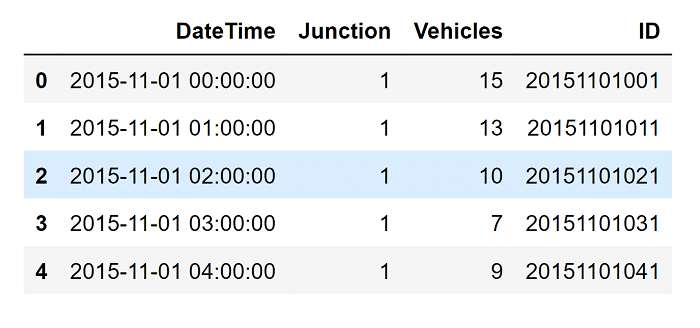

About the Data

This dataset is a compilation of hourly counts of automobiles at four intersections. There are four features in the CSV file:

• DateTime
• Junctions
• Vehicles
• ID

The traffic data comes from several time periods since the sensors on each of these intersections were gathering data at different times. Data from several of the intersections were scarce or restricted.

Data Exploration

• Feature engineering for EDA
• Plotting time series
• Parsing dates

Output: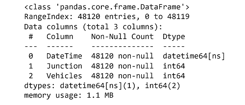

Output:

Text(0.5, 0, 'Date')

Notable details in the plot above:

• Here, it is clear that the first junction is clearly trending higher.
• Data for the fourth junction are scarce and only available after 2017.
• The aforementioned storyline does not include any mention of the season; thus, in order to learn more about it, we must look into datetime composition.

Feature Engineering

At this stage, We are using DateTime to build a few additional functionalities. Namely:

• Year
• Month
• Date in the given month
• Days of week
• Hour

Output:

Exploratory Data Analysis

The newly formed features are going to be plotted now.

Output: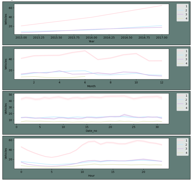

The plot described above leads to the following conclusions:

• With the exception of the fourth junction, all junctions have shown a rising yearly tendency. As was already stated above, the fourth junction contains scant data that doesn't go back more than a year.
• We can observe that around June, there is an increase in traffic at the first and second crossroads. This, we assume, may be related to summer vacation and related activities.
• There is considerable consistency in the data on a monthly basis across all dates.
• We may observe that there are peaks in the morning and evening and a fall in activity throughout the night for a given day. This is what was predicted.
• Due to fewer automobiles on the roadways on Sundays than on other days of the week, traffic flows more smoothly. The traffic is consistent from Monday through Friday.

Output:

Text(0.5, 0, 'Date')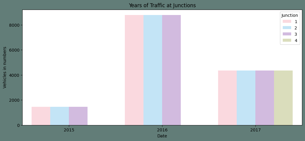

The count plot reveals that between 2015 and 2016, there was a rise in the number of automobiles. But, as we only have data for 2017 up to the seventh month, it is inconclusive to conclude the same regarding 2017.

Output: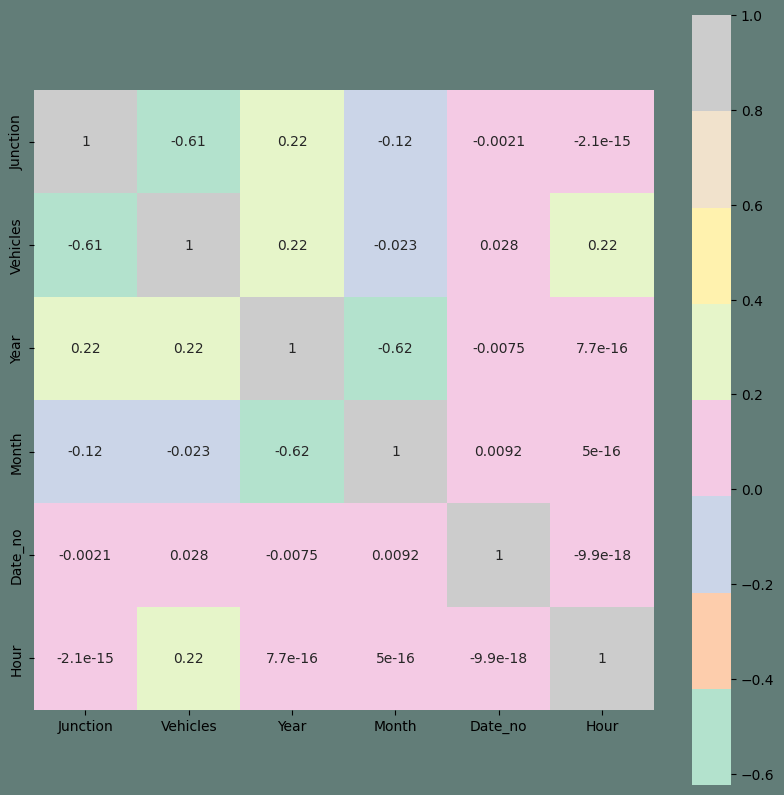

Without a doubt, the existent trait has the biggest association.

A pair plan will be used to wrap up our EDA. Any data is represented in an intriguing overall manner.

Output: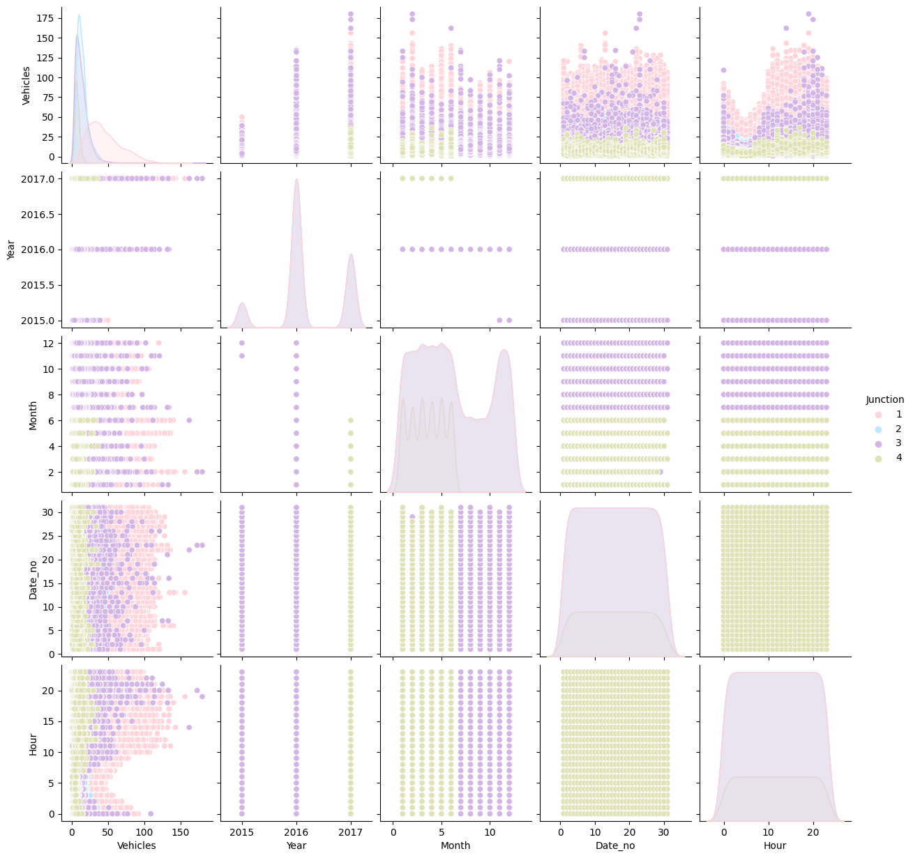

Conclusions that We've Reached After This EDA:

• Each of the four intersections has a different range of data. Just 2017's data are available for the fourth junction.
• The annual trend for Junctions 1, 2, and 3 has varying slopes.
• The first junction has a stronger weekly seasonality than the other junctions.

For the aforementioned reasons, we believe junctions should be modified to suit each one's specific requirements.

Data Transformation and Preprocessing

We shall proceed in the following order for this step:

• At each junction, make unique frames and chart them
• Plotting the series and changing it
• Using the Augmented Dickey-Fuller test to determine if converted series are seasonal
• Making training and test sets.

Output: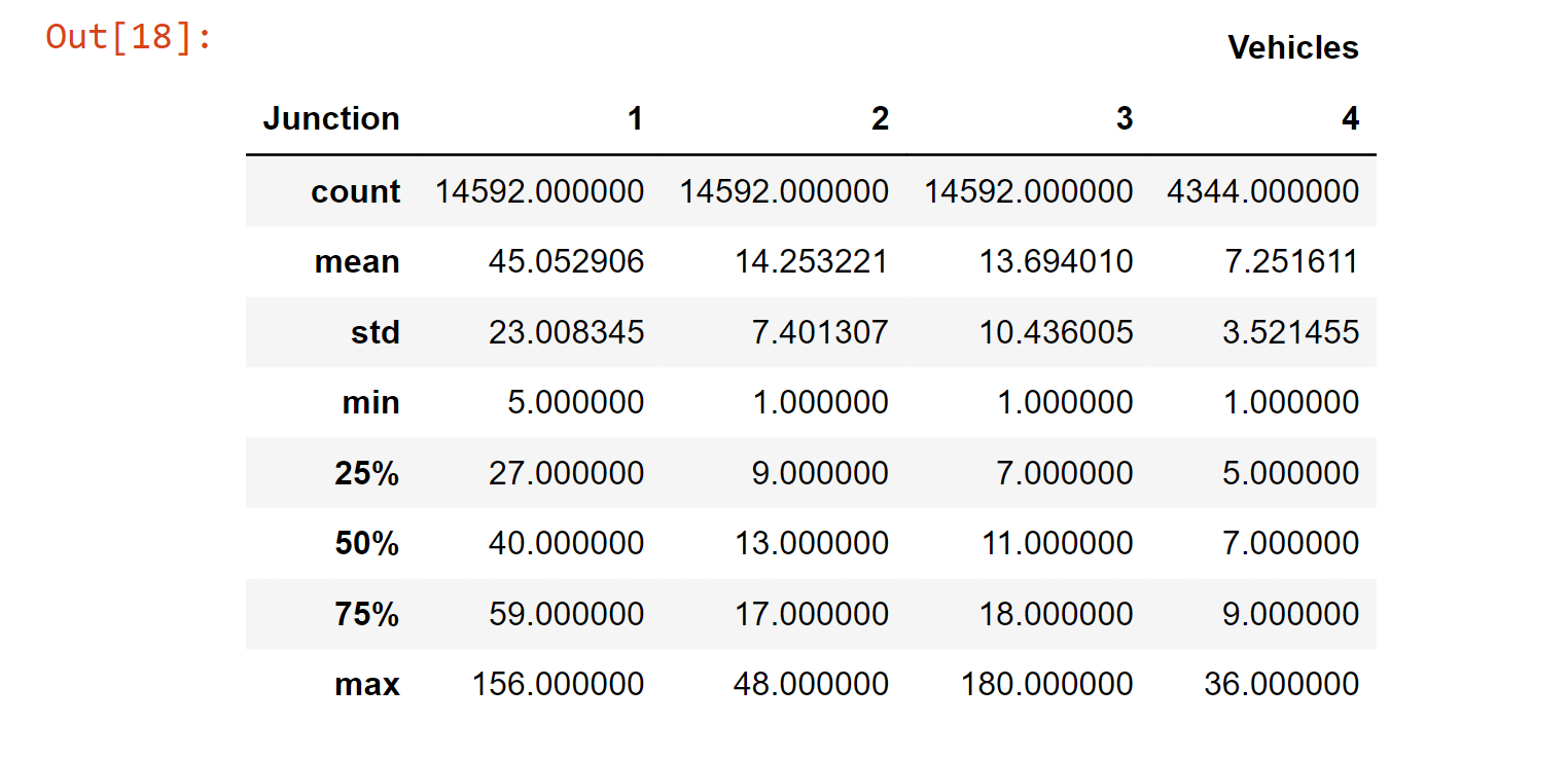

Output: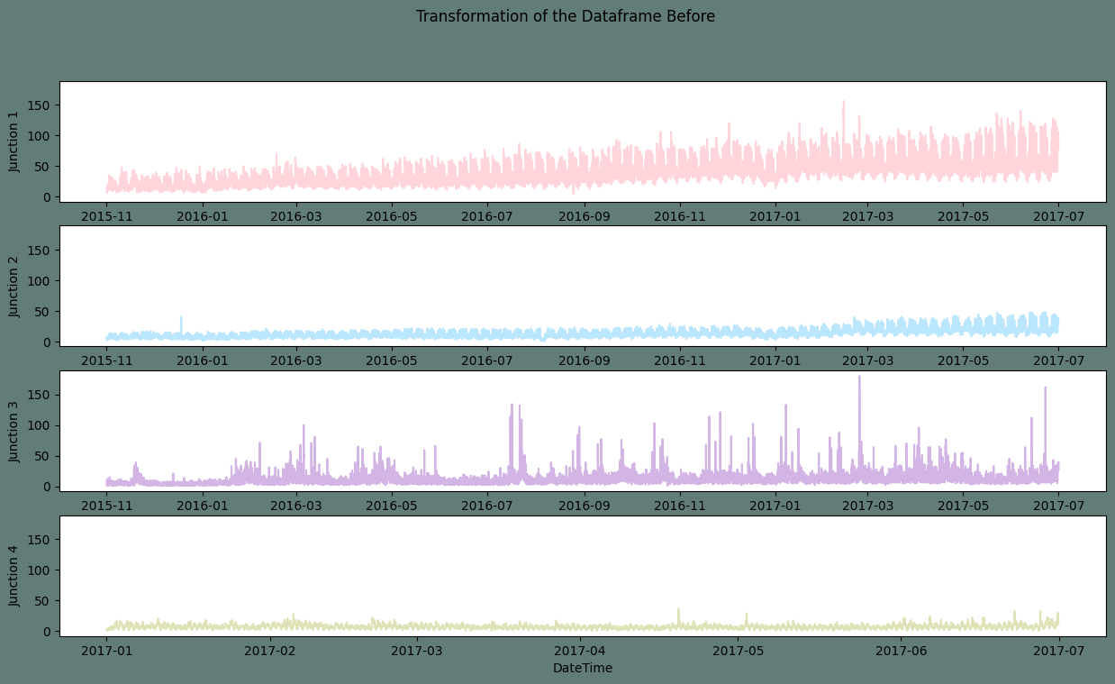

If a time series lacks a pattern or seasonality, it is said to be stagnant. Nonetheless, we observed a weekly periodicity and an increased tendency in the EDA over time. It is once again clear from the graphic above that Junctions one and two are trending higher. We will be able to notice the weekly seasonality more clearly if we restrict the span. At this time, we will skip that step and continue with the appropriate dataset transformations.

Steps for Transforming:

• Normalizing
• Differencing

In light of the aforementioned observations, the following differencing procedure should be used to remove seasonality:

• We'll be using the difference in weekly numbers for Junction 1.
• The difference of consecutive days is a preferable option for junction two.
• The difference between the hourly numbers will be used for Junctions 3 and 4.

Plots of Transformed Dataframe

Output: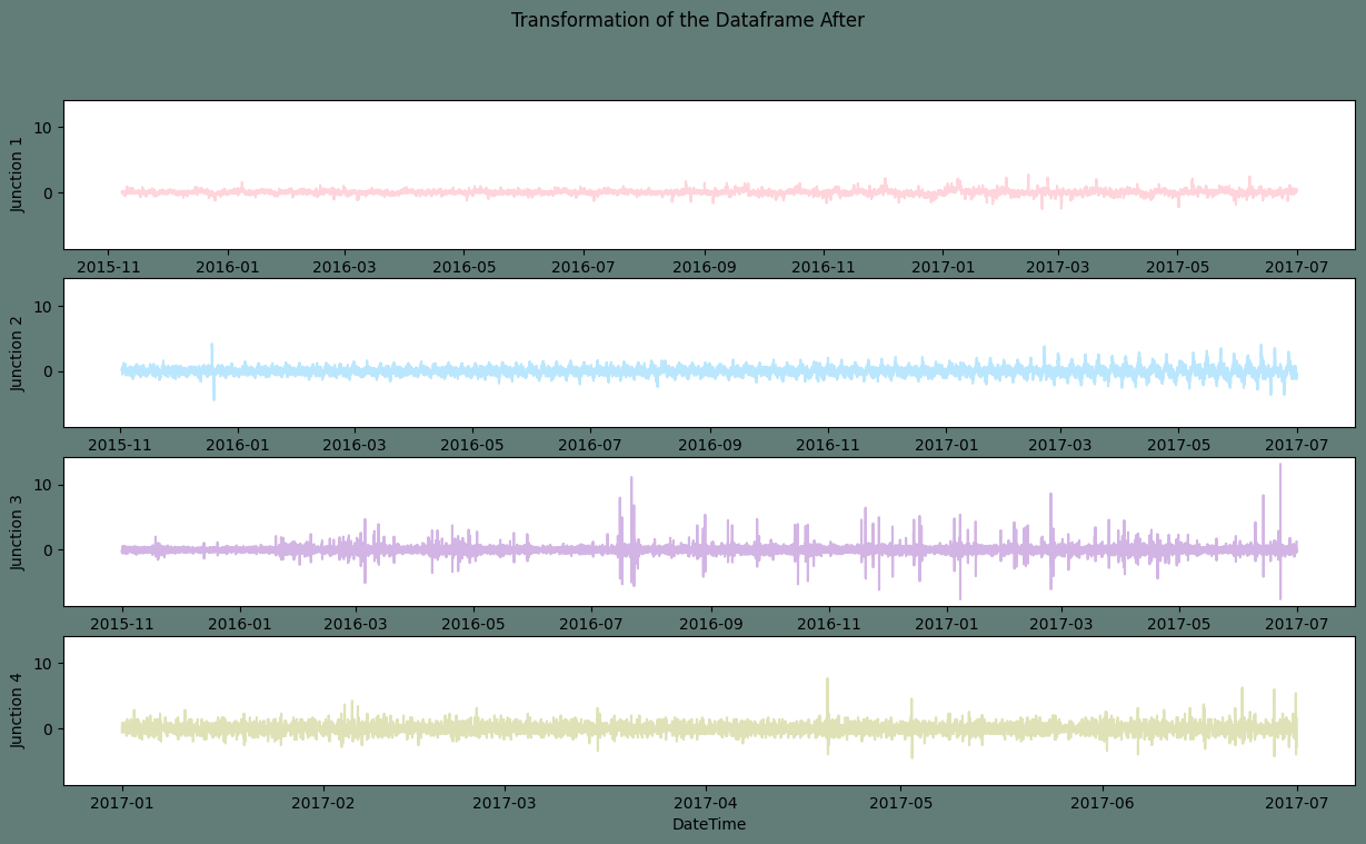

The aforementioned charts appear to be linear. An Augmented Dickey-Fuller test will be run to make sure they are stationary.

Output: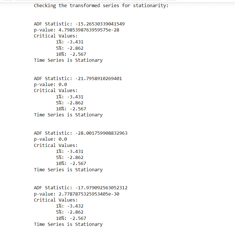

Preparing the data for the neural network :

• Splitting the test train sets
• Assigning X as features and y as target
• Reshaping data for neural net

Model Building

We have decided to employ a Gated Recurrent Unit for our project (GRU). We are developing a function in this part that the neural network may use to access and fit the data frames for all four junctions.

Fitting the Model

We will now fit the four-joint training sets that have been changed to the constructed model and contrast them with the altered test sets.

Plotting the predictions and test set while fitting the first junction

Output:

Output:

The root mean squared error is 0.245881146563882.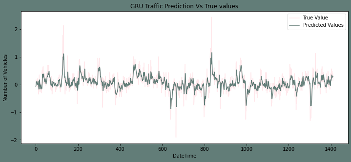

Plotting the predictions and test set while fitting the second junction

Output: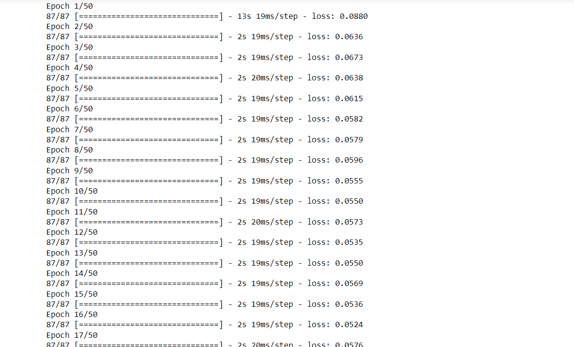

Output:

The root mean squared error is 0.5585970393765944.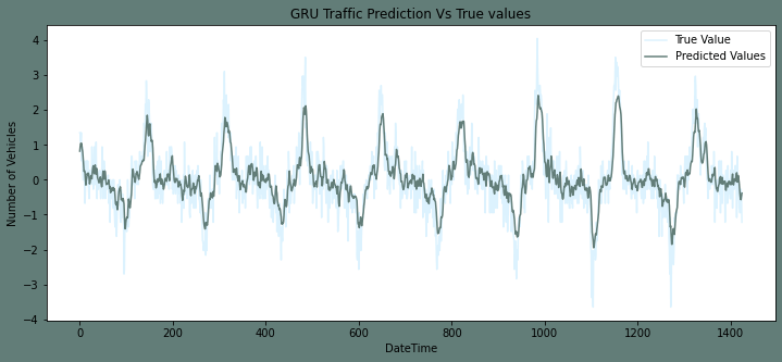

Plotting the predictions and test set while fitting the third junction

Output:

Output:

The root mean squared error is 0.6061366783632264.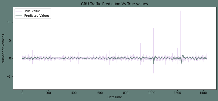

Plotting the predictions and test set while fitting the fourth junction

Output:

Output:

The root mean squared error is 1.0241982484501175.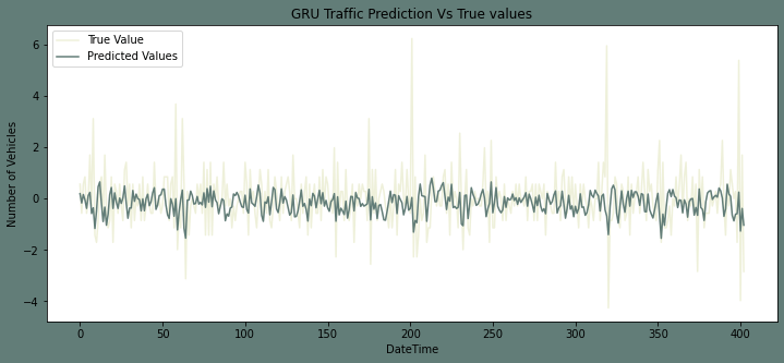

Results of the model

Output: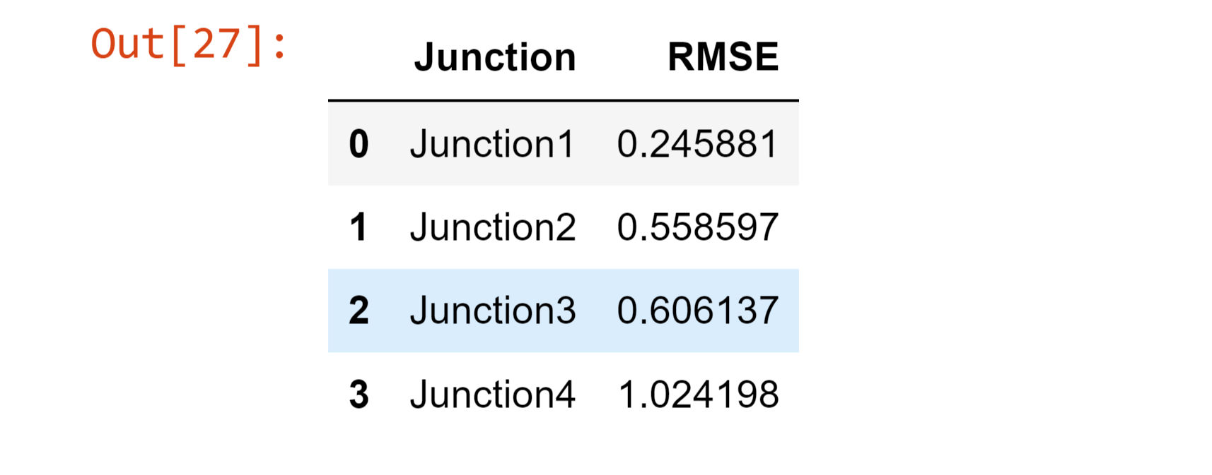

Note: The Root Mean Square Error is a very arbitrary performance indicator. As a result, we also include the outcome graphs in this project.

Inversing the Transformation of the Data

In this part, we will reverse the transformations we used to take the seasonality and trends out of the datasets. By carrying out this procedure, the forecasts will return to their previous level of accuracy.

The first junction's inverse transform

Output:

The second junction's inverse transformation

Output:

The third junction's inverse transform

Output:

The fourth junction's inverse transformation

Output:

Summary on the Dataset

Here To anticipate the traffic at four crossroads, we trained a GRU Neural network. To create a stationary time series, we employed a normalization and differentiating transform. We used a different strategy for each intersection to make it stationary because the junctions vary in trends and seasonality. We used the root mean squared error as the model's assessment measure. Also, we placed the predictions next to the initial test results. Conclusions are drawn from the data analysis:

Compared to junctions two and three, junction one is seeing a faster increase in the number of cars. Junction Four has very little data. Therefore, we can't draw any conclusions from it.

The Junction one's traffic has a stronger weekly seasonality as well as hourly seasonality. In comparison, other junctions are significantly linear.

Conclusion

In conclusion, traffic prediction using machine learning is an effective solution for addressing traffic congestion in urban areas. With the availability of vast amounts of traffic data, machine learning algorithms can accurately predict traffic flow and congestion patterns in real time. These predictions can be used to optimize traffic flow and improve the overall efficiency of transportation systems. While there are some challenges associated with traffic prediction using machine learning, the potential benefits are significant and can lead to improved transportation systems and reduced economic losses.