Betweenness Centrality (Centrality Measure)

If we want to find a node that is used as a bridge from one part of a graph to another one, we can use the betweenness centrality. Betweenness centrality can be used in graph theory so that we can measure the centrality on the basis of the shortest paths. In other words, we can say that it is used in a graph so that the un-weighted shortest paths can be calculated between all pairs of nodes. The nodes will contain higher betweenness centrality scores if those nodes frequently lie on the shortest paths between other nodes.

In a connected graph, every pair of vertices must contain a minimum of one shortest path between vertices through which we can minimize either the sum of weights of the edges (it can be only possible in a weighted graph) or the number of edges on which the path is passing (it can be only possible in the un-weighted graph). For each vertex, the betweenness centrality can be described as the number of these types of shortest paths that pass through the vertex/node.

In the network theory, there is a wide application of Betweenness centrality, i.e., It has the ability to represent the degree of nodes that stands between each other. For example, we can use it in a telecommunication network. If there is a higher betweenness centrality in a node, then that node will have more control over the network. Due to this, we can pass more information with the help of that node. The betweenness can be derived in the form of a general measure of centrality, i.e., In the network theory, we can apply it to a wide range of problems such as transport problems, social networks problems, scientific cooperation problems, and biology problems.

Definition:

The following expression is used to describe the betweenness centrality of a node v.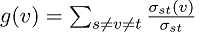

Here is used to indicate the total number of shortest paths from node s to node t.

is used to indicate the number of those paths that pass through v.

We can scale a node into the betweenness centrality with the help of a number of pairs of nodes, which can be implied by the summation indices. We can also rescale the calculation with the help of dividing the number of pairs of nodes, which does not include v in such as way that g ∈ [0, 1]. In the directed graphs, the following formula is used to perform the division:

In the undirected graph, the following formula is used to perform the division:

Here N is used to indicate the number of nodes in the giant component.

Note: We can scale any node only for the highest possible values where this node must pass by each and every single shortest path. This type of case does not often occur, and we can perform the process of normalization without a loss of precision.

This formula will generate the result as:

With the help of this formula, no precision will be lost because this formula will always be scaled from a smaller range into a larger range.

Weighted Networks

The links which are used to connect the nodes in a weighted network are now no longer treated as binary interactions. These nodes are weighted on the basis of their frequency, capacity, influence, etc. These things will be used to add another dimension of heterogeneity apart from the topological effects in the network. In a weighted network, we can find out the strength of any node with the help of doing an addition of weights of its adjacent edges. The syntax to do this is described as follows: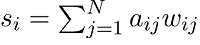

Here a_ij and w_ij are being adjacency, and they are also the weighted matrices between nodes i and j, respectively. In the scale-free network, we can find the analogous to the power-law distribution of degree. The power-law distribution is also followed by the strength of a given node.

Consideration and sampling

The resource-intensive can vary with the help of Betweenness centrality to compute many things. The single-source shortest path (SSSP) can be computed with the help of Brandes' approximate algorithm for a set of source nodes. This algorithm will generate extra results if all the nodes are selected as source nodes. In this algorithm, the runtimes will become very long for the large graphs. Thus, we can say that approximating the results with the help of computing SSSPs will be useful only for a subset of nodes. This technique will be referred to as sampling in the GDS. Here there is also sampling size which is the size of a source node set.

Suppose there are large graphs and we want to execute this algorithm. In this case, we have to consider two things, which are described as follows:

1. If there is higher parallelism, then it will lead to higher memory consumption. This is because each thread sequentially executes the single-source shortest paths (SSSPs) for a subset of source nodes. If there is any type of worst case, a single SSSP needs the entire graph to be duplicated in memory.
2. If the sampling size is higher, then we will be able to get more accurate results, but the execution process will take much longer.

Sampling strategies

There are a lot of strategies to select the source node, which is defined by Brandes. On the basis of some random degree selection strategy, the implementation of GDS is performed. In this strategy, the nodes will be selected on the basis of a probability proportional to their degree. The reason to use this strategy is that these types of nodes are likely to lie on a lot of the shortest paths in the graph. That's why this strategy will contain a higher contribution to the score of betweenness centrality.