Nature of Propositions in Discrete mathematics

If we want to learn the nature of propositions, we have to see our previous article, Propositions. Here we will show little bit about propositions.

Propositions:

Propositions can be described as declarative statements, and these statements can either be true or false but cannot be both. Propositions can be combined with the help of connectives. In this section, we are going to learn about the nature of propositions in discrete mathematics.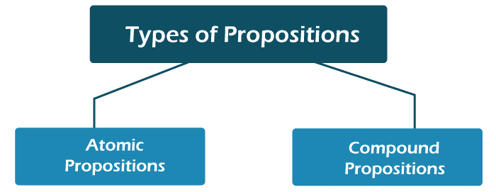

Determining Nature of Propositions

Here there is a compound proposition, and we will find out the nature of given propositions which are described as follows:

1. Tautology
2. Contradiction
3. Contingency
4. Valid
5. Invalid
6. Falsifiable
7. Unfalsifiable
8. Satisfiable
9. Unsatisfiable

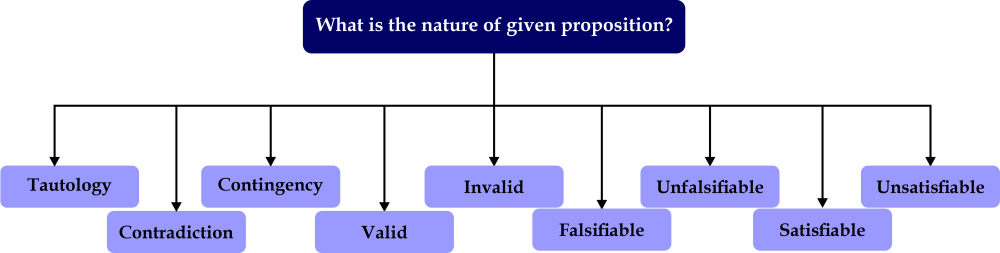
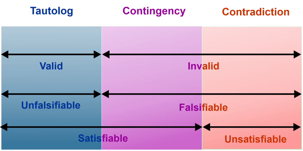
Now we will learn all of these propositions one by one.

Tautology

A compound proposition will be known as tautology iff all possible truth values of propositional variables only contain true (T). In the truth table of the tautology, the last column only has true (T).

Contradiction

A compound proposition will be known as a contradiction iff all possible truth values of propositional variables only contain false (F). In the truth table of the contradiction, the last column only has false (F).

Contingency

A compound proposition will be known as contingency iff this proposition is neither contradiction nor tautology. That means all possible truth values of propositional variables will contain both false (F) and true (T). In the truth table of the contingency, the last column has T and F both.

Valid

A compound proposition will be known as a valid proposition iff this proposition is a tautology. In the truth table of the valid, the last column only has T (Truth).

Invalid

A compound proposition will be known as an invalid proposition iff this proposition is not a tautology. That means all possible truth values of propositional variables will contain either only F(false) or both T (true) and F (false). In the truth table of the invalid, the last column either has only F or both T and F.

Falsifiable

A compound proposition will be known as falsifiable iff some values of propositional variables can make the false value. In the truth table of the falsifiable, the last column can either have F or both T and F.

Unfalsifiable

A compound proposition will be known as unfalsifiable iff any value of propositional variables cannot make the false value. In the truth table of the falsifiable, the last column can only contain the T (true).

Satisfiable

A compound proposition will be known as satisfiable iff some values of propositional variables can make the true value. In the truth table of the satisfiable, the last column can either have T or both T and F.

Unsatisfiable

A compound proposition will be known as unsatisfiable iff any value of propositional variables cannot make the true value. In the truth table of the unsatisfiable, the last column can only contain the F (false).

Important Points

There are some important points that we should know when we learn about the nature of propositions, which are described as follows:

• All contradictions will also be falsifiable and invalid, but there is no possibility of doing vice versa of it.
• All contingencies will also be falsifiable and invalid, but there is no possibility of doing vice versa of it.
• All tautologies will also be unfalsifiable and valid, and it is possible to do vice versa of it.
• All tautologies will also be satisfiable, but there is no possibility of doing vice versa of it.
• All contingencies will also be satisfiable, but there is no possibility of doing vice versa of it.
• All contradictions will also be unsatisfiable, and it is possible to do vice versa of it.

Examples of find out the Nature of Propositions

There are various examples in which we can determine the nature of propositions, which are shown below:

Example 1: In this example, we have various propositions, and we have to determine their nature.

1. x ∧ ∼x
2. (x ∧ (x → y)) → ∼y
3. [ (x → y) ∧ (y → z) ] ∧ (x ∧ ∼z)
4. ∼(x → y) ∨ (∼x ∨ (x ∧ y))
5. (x ↔ z) → (∼y → (x ∧ z))

Solution:

Here we will solve all of these propositions one by one like this:

Part 1:

We can solve the proposition x ∧ ∼x with the help of three methods, which are shown below:

Method 1: In this method, we will use the truth table like this:

In the above truth table, we can see that the last columns only have the false value (F).

Hence, this proposition can be:

• Falsifiable
• Contradiction
• Unsatisfiable
• Invalid

Method 2: In this method, we will use the Algebra of Propositions like this:

As we know that the given proposition is x ∧ ∼x.

When we apply the complement law to this proposition, then we will get x ∧ ∼x = F.

Hence this proposition can be:

• Falsifiable
• Contradiction
• Unsatisfiable
• Invalid

Method 3: In this method, we will use the Digital Electronics

In the case of digital electronics, we can write the given proposition as x.x'.

Clearly, we can say that x.x' = 0.

Hence, this proposition can be:

• Invalid
• Unsatisfiable
• Contradiction
• Falsifiable

Part 2:

We can solve the (x ∧ (x → y)) → ∼y with the help of three methods, which are shown below:

Method 1: In this method, we will use the truth table like this:

In the above truth table, we can see that the last columns have both false values (F) and truth values (T).

Hence, this proposition can be:

• Falsifiable
• Contingency
• Satisfiable
• Invalid

Method 2: In this method, we will use the Algebra of Propositions like this:

(x ∧ (x → y)) → ∼y

= (x ∧ (∼x ∨ y)) → ∼y {∵ x → y = ∼x ∨ y}

= ∼(x ∧ (∼x ∨ y)) ∨ ∼y {∵ x → y = ∼x ∨ y}

Now we will use the distributive law like this:

= ∼((x ∧ ∼x) ∨ (x ∧ y)) ∨ ∼y

Now we will use the complement law like this:

= ∼(F ∨ (x ∧ y)) ∨ ∼y

Now we will use the identity law like this:

= ∼(x ∧ y) ∨ ∼y

Now we will use the De Morgans law like this:

= ∼x ∨ ∼y ∨ ∼y

= ∼x ∨ ∼y

Clearly, we can see that the result is neither T nor F.

Hence this proposition can be:

• Falsifiable
• Contingency
• Satisfiable
• Invalid

Method 3: In this method, we will use the Digital Electronics

We have the following:

= (x ∧ (x → y)) → ∼y

= (x ∧ (∼x ∨ y)) → ∼y {∵ x → y = ∼x ∨ y}

= ∼(x ∧ (∼x ∨ y)) ∨ ∼y {∵ x → y = ∼x ∨ y}

Now we have the following in terms of digital electronics:

= (x. (x' + y))' + y'

= (x.x' + x.y)' + y'

= (x.y)' + y' {∵ x.x' = 0}

Now we will use De Morgan's law like this:

= x' + y' + y'

= x' + y'

Clearly, we can say that the result is neither 0 nor 1.

Hence, this proposition can be:

• Falsifiable
• Contingency
• Satisfiable
• Invalid

Part 3:

We can solve the [(x → y) ∧ (y → z)] ∧ (x ∧ ∼z) with the help of three methods, which are shown below:

Method 1: In this method, we will use the truth table like this:

Here we will assume that [(x → y) ∧ (y → z)] ∧ (x ∧ ∼z) = R (say)

In the above truth table, we can see that the last column only has false values (F).

Hence, this proposition can be:

• Falsifiable
• Contradiction
• Unsatisfiable
• Invalid

Method 2: In this method, we will use the Algebra of Propositions.

We have the following:

[(x → y) ∧ (y → z)] ∧ (x ∧ ∼z)

= [ (∼x ∨ y) ∧ (∼y ∨ z) ] ∧ (x ∧ ∼z) {∵ x → y = ∼x ∨ y}

Now we will use the distributive law like this:

= [((∼x ∨ y) ∧ ∼y) ∨ ((∼x ∨ y) ∧ z)] ∧ (x ∧ ∼z)

Now we will again use the distributive law like this:

= [((∼x ∧ ∼y) ∨ (y ∧ ∼y)) ∨ ((∼x ∧ z) ∨ (y ∧ z))] ∧ (x ∧ ∼z)

Now we will use the complement law like this:

= [((∼x ∧ ∼y) ∨ F) ∨ ((∼x ∧ z) ∨ (y ∧ z))] ∧ (x ∧ ∼z)

Now we will use the Identity law like this:

= [(∼x ∧ ∼y) ∨ (∼x ∧ z) ∨ (y ∧ z)] ∧ (x ∧ ∼z)

Now we will use distributive law like this:

= ((∼x ∧ ∼y) ∧(x ∧ ∼z)) ∨ ((∼x ∧ z) ∧(x ∧ ∼z)) ∨ ((y ∧ z) ∧ (x ∧ ∼z))

= (∼x ∧ ∼y ∧ x ∧ ∼z) ∨ (∼x ∧ z ∧ x ∧ ∼z) ∨ (y ∧ z ∧ x ∧ ∼z)

Now we will use the complement law like this:

= F ∨ F ∨ F

= F

Clearly, we can say that the result of this proposition is F.

Hence, this proposition can be:

• Falsifiable
• Contradiction
• Unsatisfiable
• Invalid

Method 3: In this method, we will use the Digital Electronics

We have the following:

[(x → y) ∧ (y → z)] ∧ (x ∧ ∼z)

= [(∼x ∨ y) ∧ (∼y ∨ z) ] ∧ (x ∧ ∼z) {∵x→ y = ∼x ∨ y}

Now we have the following in terms of digital electronics:

= [(x' + y) . (y' + z) ] . (x.z')

= [x'. y' + x'.z + y.y' + y.z] . (x.z')

= [x'.y' + x'.z + 0 + y.z] . (x.z') {∵ y.y' = 0}

= [x'.y' + x'.z + y.z] . (x.z')

= x'.y'.x.z' + x'.z.x.z' + y.z.x.z'

= 0 + 0 + 0

= 0

Clearly, we can say that the result is 0.

Hence, this proposition can be:

• Falsifiable
• Contradiction
• Unsatisfiable
• Invalid

Part 4:

We can solve the ∼(x → y) ∨ (∼x ∨ (x ∧ y)) with the help of three methods, which are shown below:

Method 1: In this method, we will use the truth table like this:

Here we will assume that ∼(x → y) ∨ (∼x ∨ (x ∧ y)) = R (say)

In the above truth table, we can see that the last column only has the true values (T).

Hence, this proposition can be:

• Unfalsifiable
• Tautology
• Satisfiable
• Valid

Method 2: In this method, we will use the Algebra of Propositions.

We have the following:

∼(x → y) ∨ (∼x ∨ (x ∧ y))

= ∼(∼x ∨ y) ∨ (∼x ∨ (x ∧ y)) {∵ x → y = ∼x ∨ y}

Now we will use the De Morgans law like this:

= (x ∧ ∼y) ∨ (∼x ∨ (x ∧ y))

Now we will use the distributive law like this:

= (x ∧ ∼y) ∨ ((∼x ∨ x) ∧ (∼x ∨ y))

Now we will use the Complement law like this:

= (x ∧ ∼y) ∨ (T ∧ (∼x ∨ y))

Now we will use the Identity law like this:

= (x ∧ ∼y) ∨ (∼x ∨ y)

Now we will use the Associative law like this:

= ((x ∧ ∼y) ∨ ∼x) ∨ y

Now we will use the Distributive law like this:

= ((x ∨ ∼x) ∧ (∼y ∨ ∼x)) ∨ y

Now we will use the Complement law like this:

= (T ∧ (∼y ∨ ∼x)) ∨ y

Now we will use the Identity law like this:

= (∼y ∨ ∼x) ∨ y

= ∼x ∨ (y ∨ ∼y)

Now we will use the Complement law like this:

= ∼x ∨ T

Now we will use the Identity law like this:

= T

Clearly, we can say that the result of this proposition is T.

Hence, this proposition can be:

• Unfalsifiable
• Tautology
• Satisfiable
• Valid

Method 3: In this method, we will use the Digital Electronics

We have the following:

[(x → y) ∧ (y → z)] ∧ (x ∧ ∼z)

= [(∼x ∨ y) ∧ (∼y ∨ z) ] ∧ (x ∧ ∼z) {∵x→ y = ∼x ∨ y}

Now we have the following in terms of digital electronics:

= (x' + y)' + (x' + x.y)

Now we will use the Transposition theorem like this:

= (x' + y)' + (x' + x).(x' + y)

= (x' + y)' + 1.(x' + y)

= (x' + y)' + (x' + y)

Now we will use the De Morgans law like this:

= x.y' + x' + y

Now we will use the Transposition theorem like this:

= (x + x')(x' + y') + y

= 1.(x' + y') + y

= x' + (y' + y)

= x' + 1

= 1

Clearly, we can say that the result of this proposition is 1.

Hence, this proposition can be:

• Unfalsifiable
• Tautology
• Satisfiable
• Valid

Part 5:

We can solve the (x ↔ z) → (∼y → (x ∧ z)) with the help of three methods, which are shown below:

Method 1:

In this method, we will use the truth table like this:

Here we will assume that (x ↔ z) → (∼y → (x ∧ z)) = R (say)

In the above truth table, we can see that the last column has both true values (T) and false values (F).

Hence, this proposition can be:

• Falsifiable
• Satisfiable
• Invalid
• Contingency

Method 2: In this method, we will use the Algebra of Propositions.

We have the following:

(x ↔ z) → (∼y → (x ∧ z))

= (x ↔ z) → (y ∨ (x ∧ z)) {∵ x → y = ∼x ∨ y}

= ∼(x ↔ z) ∨ y ∨ (x ∧ z)

= ∼((x → z) ∧ (z → x)) ∨ y ∨ (x ∧ z) {∵ x ↔ y = (x → y) ∧ y → x)}

= ∼((∼x ∨ z) ∧ (∼z ∨ x)) ∨ y ∨ (x ∧ z) {∵ x → y = ∼x ∨ y}

Now we will use the Distributive law like this:

= ∼[ ((∼x ∨ z) ∧ ∼z) ∨ ((∼x ∨ z) ∧ x) ] ∨ y ∨ (x ∧ z)

Now we will again use the Distributive law like this:

= ∼[((∼x ∧ ∼z) ∨ (z ∧ ∼z)) ∨ ((∼x ∧ x) ∨ (z ∧ x)) ] ∨ y ∨ (x ∧ z)

Now we will use the Complement law like this:

= ∼[((∼x ∧ ∼z) ∨ F) ∨ (F ∨ (z ∧ x)) ] ∨ y ∨ (x ∧ z)

Now we will use the Identity law like this:

= ∼[(∼x ∧ ∼z) ∨ (z ∧ x) ] ∨ y ∨ (x ∧ z)

Now we will use the De Morgans law like this:

= [∼(∼x ∧ ∼z) ∧ ∼(z ∧ x) ] ∨ y ∨ (x ∧ z)

Now we will again use the De Morgans law like this:

= [(x ∨ z) ∧ (∼z ∨ ∼x) ] ∨ y ∨ (x ∧ z)

Now we will use the Distributive law like this:

= ((x ∨ z) ∧ ∼z) ∨ ((x ∨ z) ∧ ∼x) ∨ y ∨ (x ∧ z)

Now we will again use the Distributive law like this:

= ((x ∧ ∼z) ∨ (z ∧ ∼z)) ∨ ((x ∧ ∼x) ∨ (z ∧ ∼x)) ∨ y ∨ (x ∧ z)

Now we will use the Complement law like this:

= ((x ∧ ∼z) ∨ F) ∨ (F ∨ (z ∧ ∼x)) ∨ y ∨ (x ∧ z)

Now we will use the Identity law like this:

= (x ∧ ∼z) ∨ (z ∧ ∼x) ∨ y ∨ (x ∧ z)

= (x ∧ ∼z) ∨ y ∨ (∼x ∧ z) ∨ (x ∧ z)

Now we will use the Distributive law like this:

= (x ∧ ∼z) ∨ y ∨ ((∼x ∨ x) ∧ z)

Now we will use the Complement law like this:

= (x ∧ ∼z) ∨ y ∨ (T ∧ z)

Now we will use the Identity law like this:

= (x ∧ ∼z) ∨ y ∨ z

= z ∨ (x ∧ ∼z) ∨ y

Now we will use the Distributive law like this:

= ((z ∨ x) ∧ (z ∨ ∼z)) ∨y

Now we will use the Complement law like this:

= ((z ∨ x) ∧ T) ∨ y

Now we will use the Identity law like this:

= x ∨ y ∨ z

Clearly, we can say that the result of this proposition is neither T nor F.

Hence, this proposition can be:

• Falsifiable
• Satisfiable
• Invalid
• Contingency

Method 3: In this method, we will use the Digital Electronics

We have the following:

(x ↔ z) → (∼y → (x ∧ z))

= (x ↔ z) → (y ∨ (x ∧ z)) {∵x → y = ∼x ∨ y}

= ∼(x ↔ z) ∨ (y ∨ (x ∧ z)) {∵x → y = ∼x ∨ y}

Now we have the following in terms of digital electronics:

= (x.z + x'.z')' + (y + x.z)

Now we will use the De Morgans Theorem like this:

= (x.z)' . (x'.z')' + (y + x.z)

Now we will again use the De Morgans Theorem like this:

= (x' + z') . (x + z) + (y + x.z)

= x'.x + x'.z + z'.x + z'.z + y + x.z

= 0 + x'.z + z'.x + 0 + y + x.z

= x'.z + z'.x + y + x.z

= (x' + x).z + z'.x + y

= z + z'.x + y

Now we will use the Transposition Theorem like this:

= (z + z').(z + x) + y

= x + y + z

Clearly, we can say that the result of this proposition is neither 0 nor 1.

Hence, this proposition can be:

• Falsifiable
• Satisfiable
• Invalid
• Contingency