Sampling and Inference

A sample is defined as a method of selecting a small section from a population or large data. The process of drawing a sample from large data is known as sampling. It is used in various applications, such as mathematics, digital communication, etc.

It is essential that a selected sample must be random selection so that each member has an equal chance to appear in the selection process. Thus, the fundamental assumption based on the sampling is called random sampling.

Here, we will discuss the following:

Sampling Distribution

Testing of Hypothesis

Level Significance

Comparison of two samples

Student t-distribution

Central Limit Theorem

Chi-Square Method

F Distribution

Sampling Distribution

We generally compute the mean of n number of samples taken from the population. The means of various samples are different. If these different means are grouped according to their frequencies, it is termed as the sampling distribution of the mean. Similarly, if we group these different standard deviations according to their frequencies, it is termed as the sampling distribution of the standard deviation.

Simple Sampling

It is a special case of random sampling. Here, each event has the same probability of success, which is independent of each other. It means that the occurrence of one does not depend on the occurrence of the other and their previous trials. The statistical parameters of the population are mean and standard deviation.

Why sampling is important?

Sampling aims at collecting maximum information within minimum time, cost, and efforts. It obtains the best possible values. According to the sampling logic of induction, a particular sample is passed to the general population. Such a generalization from a sample to the population is termed as statistical inference.

Attributes of Sampling

The probability of success = p

The probability of failure = q = (1 - p)

Suppose we draw the samples with n number of independent trials. The occurrence of a outcome does not depend on the occurrence of the other.

Binomial expression = (p + q)ⁿ

Mean = np

SD (Standard Deviation) = √npq

The expected value of success in a sample of size n is np and the standard error is √npq.

Let's consider the proportion of success.

The means proportion of success = np/n = p

Standard error of the proportion of success = √(n x p/n x q/n) = √(pq/n)

Precision of the proportion of success = √(n/pq)

Precision is the reciprocal of the standard error.

It depends on √n because p and q are constants.

Standard Error

The standard error is defined as the difference between the expected value and the observed value. If n is greater than 30, the sample is known as a large sample. Otherwise, the sample is small. The standard error of the sampling distribution of the mean is called the standard error of the mean, and the standard error of the sampling distribution of SD is called the standard error of SD.

Testing of Hypothesis

Testing a hypothesis means testing whether the hypothesis is true or false. At first, the hypothesis is assumed as correct, and the probability is calculated. The hypothesis is rejected when the probability calculated is less than the preassigned value.

Errors

Errors arises when the hypothesis is rejected or accepted instead of accepted or rejected. There are two types of errors, Type I error and Type II error.

Type I error: If the hypothesis is rejected instead of being accepted, the error is termed as Type I error.

Type II error: If the hypothesis is accepted instead of being rejected, the error is termed as Type II error.

The aim of testing a hypothesis is to minimize the type II error and limit the type I error to the preassigned value of 5% or 1%. The best method to reduce both type of errors (Type I and II) is to increase the sample size.

Null Hypothesis: It is denoted by H_o. Accepting a null hypothesis based on statistical data signifies that the hypothesis is not rejected. It does not mean that the hypothesis is true, nor does it mean that it is false.

Level Significance

The level of probability below which a certain hypothesis is rejected, is known as the level of significance. There are two values accepted for the level of significance, i.e. 5% and 1%. The procedure that allows us to test the acceptance or rejection of the hypothesis is known as the testing of significance. We generally test the difference between the sample values and the population values.

We know that for the binomial distribution of n samples, the formula to calculate the mean and standard deviation is given by:

Mean = np

SD (Standard Deviation) = √npq

Where,

p is the probability of success

n is the probability of failure

We have the following conditions to test the level of significance,

|z| < 1.96, the difference is not significant

|z| > 1.96, the difference is at 5% level of significance

|z| > 2.58, the difference is at 1% level of significance

Where,

Z is the standard normal variate

Z = (x - u)/ σ

Or

Z = (x -mean)/SD

Z = (x - np)/√npq

X is the value for observed number of successes.

The difference is calculated on the basis of expected and observed number of successes.

Numerical Examples

Let's discuss some numerical examples based on testing of level significance.

Example 1:

A coin was tossed 200 times with 108 number of heads. Test the hypothesis that the coin is biased at 5% level of significance?

Solution:

Let's consider the above coin as unbiased.

The probability of getting a head = 1/2

n = 1/2

The probability of getting a tail = 1/2

p = 1/2

Thus, the probability of getting a head is the probability of success.

The expected number of successes = 1/2 x 200

= 100

The observed value of successes = 108

Difference = Observed value of success - expected value of success

Difference = 108 - 100

Difference = 8

Standard Deviation = √npq

= √200 x ½ x ½

= √50

= 7.07

Z = (x - np)/√npq

Z = 8/7.07

Z = 1.13

Z < 1.96

The value of z is less than 1.96. Hence, the hypothesis of the unbiased coin is accepted at 5% level of significance.

Example 2:

A die is thrown 12000 times and the throw of 2 or 3 was obtained 5400 times? On the basis of random dice throwing, does the data indicate the biased or unbiased die?

Solution:

Let's consider the above coin as unbiased.

The probability of getting 2 or 3= 1/3

n = 1/3

The probability of not getting 2 or 3 = (1 - 1/3)

p = 2/3

The expected number of successes = 1/3 x 12000

= 4000

The observed value of successes = 5400

Difference = Observed - expected number of successes

= 5400 - 4000

= 1400

Standard Deviation = √npq

= √(12000 x 1/3 x 2/3)

= 51.63

Z = (x - np)/√npq

Z = 1400/51.63

Z = 27.11

Z > 2.58

The value of z is greater than 2.58. Hence, the hypothesis of the biased coin is rejected at 1% level of significance.

Comparison of two Samples

We have discussed the hypothesis and testing of level significance of a sample n taken from the population p. Here, we will discuss two large samples of size n₁ and n₂ taken from the population's p1 and p2. We combine the two samples to find the estimate value of proportion, which is given by:

P = (n₁p₁ + n₂p₂)/ (n₁ + n₂)

The standard errors E₁ and E₂ are given by:

E₁² = pq/ n₁

E₂² = pq/ n₂

E² = E₁² + E₂²

E² = pq (1/ n₁ + 1/n₂)

Z = (p₁ - p₂)/ E

Z is the standard normal variate

If z > 3, the difference is real

If z < 2, the difference is fluctuating

If the value of z lies between 2 and 3, the difference between p₁ and p₂ is significant at 5% level of significance.

Numerical Examples

Let's discuss three numerical examples based on the comparison of samples.

Example 1:

In city P, 25% of samples of 1000 girls has a certain physical defect. In another city Q, 20% of samples of 800 girls has the same defect. Find if the difference between the two propagations is significant?

Solution:

n₁ = 1000

n₂ = 800

p₁ = 25% = 25/100 = 1/4

p₂ = 20% = 20/100 = 1/5

The estimate value of proportion is given by:

P = (n₁p₁ + n₂p₂)/ (n₁ + n₂)

P = (250 + 160)/1800

P = 310/1800

P = 0.17

Q = 1 - P

Q = 0.83

E² = pq (1/ n₁ + 1/n₂)

E² = 0.17 x 0.83 (1/1000 + 1/800)

E² = 0.1411 (0.00225)

E = 0.0178

E = 0.02 (approx.)

p₁ - p₂ = 25% - 20%

= 5%

= 5/100

= 0.05

Z = (p₁ - p₂)/ E

Z = 0.05/0.02

Z = 2.5

The value of Z lies between 2 and 3. Hence, the value is significant at 5% level of significance.

Example 2:

In city A, 11% of samples of 500 boys has a certain physical defect. In another city B, 10% of samples of 600 boys has the same defect. Find if the difference between the two propagations is significant?

Solution:

n₁ = 500

n₂ = 600

p₁ = 11% = 11/100 = 0.11

p₂ = 10% = 10/100 = 0.1

The estimate value of proportion is given by:

P = (n₁p₁ + n₂p₂)/ (n₁ + n₂)

P = (55 + 60)/1100

P = 115/1100

P = 0.105

Q = 1 - P

Q = 0.89

E² = pq (1/ n₁ + 1/n₂)

E² = 0.11x 0.89 (1/500 + 1/600)

E² = 0.0979 (0.00367)

E = 0.019

p₁ - p₂ = 11% - 10%

= 1%

= 1/100

= 0.01

Z = (p₁ - p₂)/ E

Z = 0.01/0.019

Z = 0.52

Z < 1

The value of Z is less than 1. Hence, the difference between proportions in not significant.

Example 3:

In two large populations, there are 35% and 30% of the people with small height. Find if the difference is likely to hidden in the 1000 and 700 samples from these two populations?

Solution:

p₁ = 0.35 or 35%

p₂ = 0.30 or 30%

q₁ = (1 - p₁)

q₁ = 0.65

q₂ = (1 - p₂)

q₂ = 0.7

p₁ - p₂ = 35% - 30%

p₁ - p₂ = 5%

p₁ - p₂ = 5/100

p₁ - p₂ = 0.05

E² = p₁q₁ / n₁ + p₂q₂ /n₂

E² = 0.35 x 0.65 /1000 + 0.30 x 0.70/ 700

E² = 0.0002275 + 0.0003

E² = 0.0005275

E = 0.02296

Z = (p₁ - p₂)/ E

Z = 0.05/0.02296

Z = 2.18

It is unlikely that the real difference will be hidden.

Central Limit Theorem

Central Limit Theorem is useful in the distribution of mean samples for the large sample size.

The limiting distribution of a sample size of n is given by:

Z = (x - u)/ (σ /√n)

Where,

u is the mean

σ is the Standard Deviation

The distribution has a finite mean and standard distribution. The samples with a size greater than 25 are termed as large samples.

Central limit theorem is universal and focuses on the normal distribution in statistical theory.

Examples

Here, we will discuss two examples based on the central limit theorem.

Example 1: A sample of 900 bottles has a mean of 3.8. Can it be regarded as a true sample from a large population with a mean 3.6 and a standard deviation 1.51?

Solution:

x = 3.8

u = 3.6

σ = 1.51

n = 900

Z = (x - u)/ (σ/ √n)

Z = (3.8 - 3.6)/1.51 /(30)

Z = 0.2/1.51/ (30)

Z = 0.2 x 30 /1.51

Z = 3.977

Z > 1.96

The value of Z is greater than 1.96. Hence, the mean of the population is significant at 5% level of significance.

Example 2: A sample of 400 members has a mean of 2.24. Can it be regarded as a true sample from a large population with the mean 2.2 and a standard deviation 0.51?

Solution:

x = 2.24

u = 2.2

σ = 0.51

n = 400

Z = (x - u)/ (σ/ √n)

Z = (2.24 - 2.2)/0.51/ (20)

Z = 0.04/0.51/ (20)

Z = 0.04 x 20 /0.51

Z = 1.57

Z < 1.96

The value of Z is less than 1.96. Hence, the mean of the population is not significant.

Test of significance of mean for two large samples

Here, we will discuss two large samples of size n₁ and n₂ taken from the population with mean u₁ and u₂ and the standard deviation σ₁ and σ₂.

The standard error of mean for these two samples is given by:

E = σ √(1/ n₁ + 1/n₂)

Z = x₁ - x₂/E

Z = x₁ - x₂/ σ √(1/ n₁ + 1/n₂)

Test of significance

The condition to test the significance are as follows:

If z > 1.96, the difference is significant a 5% level of significance.

If z > 3, either the sampling is not simple or the drawn samples are not from the same population.

Examples

Example 1: The mean of sample of size 500 and 1000 are 45.5 and 46. Can the samples regarded as drawn from the population with a standard deviation of 1.5.

Solution:

x₁ = 45.5

x₂ = 46

n₁ = 500

n₂ = 1000

Z = x₁ - x₂/ σ √(1/ n₁ + 1/n₂)

Z = 0.5/ 1.5 x √(1/500 + 1/1000)

Z = 0.5/ 1.5 x √ (0.003)

Z = 0.5/0.082

Z = 6.09

The difference is much higher. Hence, the samples cannot be regarded as the samples drawn from the population.

Example 2: The mean of sample of size 800 and 1600 are 50 and 50.4. Can the samples regarded as drawn from the population with a standard deviation of 3.5.

Solution:

x₁ = 50

x₂ = 50.4

n₁ = 800

n₂ = 1600

Z = x₁ - x₂/ σ √(1/ n₁ + 1/n₂)

Z = 0.4/ 3.5 x √(1/800 + 1/1600)

Z = 0.4/ 3.5 x √ (0.001875)

Z = 0.4/0.152

Z = 2.63

The difference is greater than 1.96 and less than 3. Thus, the difference is significant at 5% level of significance.

Student's T-distribution

The statistical t in the student's t-distribution is given by:

t = (x - u)/ σ√n

or

t = (x - u)/ σ_s√(n - 1)

Where,

u is the mean

σ is the Standard Deviation

σ_s is the Sample Standard Deviation

The student's t-distribution can be expressed as:

Y = y_o/(1 + t²/v)^{(v + 1)/2}

Where,

y_o is the constant

v = n - 1

The t-curve is shown below: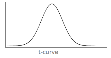

The area under the t-curve is unity. The normal curve approaches the horizontal axis faster than the t-curve. The t-curve attains the maximum value at t= 0 in order to make the mode coincides with the mean.

The prescribed level of significance is taken from the table V.

Examples

Let's discuss two examples based on the student's t-distribution.

Example 1: A random samples of 12 patients shows the data of the increase in the blood pressure 5, 4, 3, -2, 0, 1, -1, 8, 7, 2, 1, 4.

Solution:

Mean = 5 + 4 + 3 -2 + 0 + 1 -1 + 8 + 7 + 2 + 1 + 4/12

Mean = d' = 2.67

σ ² = Σd²/n - d'²

σ ² = 1/12 (25 + 16 + 9 + 4 + 0 + 1 + 1 + 64 + 49 + 4 + 1 + 16) - 2.67

σ ² = 1/12 (190) - 2.67

σ ² = 13.16

σ = 3.62

t = (d - u)/ σ_s√(n - 1)

u = 0

t = (2.67 - 0)/ 3.62 x √11

t = 0.737 x √11

t = 2.45

v = n - 1 = 12 - 1 = 11

t_0.05 for v = 11 is equal to 2.2 from table V.

|t| > t_0.05

The value of t is greater than t0.05. Hence, our assumption is rejected.

We can access the table C direct from the link https://www.sjsu.edu/faculty/gerstman/StatPrimer/t-table.pdf.

Example 2: The nine items in a basket has a sample value of 25, 27, 30, 32, 28, 27, 29, 33, and 31. Does the mean of these nine items differ significantly from the assumed mean of 27.5?

Solution:

Mean = x + Σd/n

Mean = 28 + 10/9

Mean = 29.1

Sample standard deviation σ _s = Σd²/n - (Σd/n)²

σ _s² = 66/9 - 100/81

σ _s = 2.47

t = (d - u)/ σ_s√(n - 1)

t = (29.1 - 27.5)/ 2.47 x √8

t = 0.647 x √8

t = 1.83

v = n - 1 = 9 - 1 = 8

t_0.05 for v = 8 is equal to 2.31 from table V.

|t| < t_0.05

The value of t is less than t_0.05. Hence, it is not significant at 5% level of significance.

Example 3: The table shows the data of 11 students in two tests. The second test was taken one month after the first test. Find if there is any improvement in the performance of students in the second test?

Solution:

d' = 11/11 = 1

σ _s² = Σ (d - d')²/(n - 1)

σ _s² = 104/10

σ _s² = 10.4

σ _s = 3.22

v = n - 1 = 11 - 1 = 10

t_0.05 for v = 10 is equal to 2.228 from table V.

|t| < t_0.05

The value of t is greater than t0.05. Hence, our assumption is rejected.

Chi-Square Method

When a coin is tossed 60 times, the theoretical expectations are 30 heads and 30 tails. But in practical, it is not possible. The outcomes of an experiment are not same as the theoretical outcomes. The magnitude of the difference between the observation and theory is defined as chi-square and is represented as X².

When X² = 0, the observed outcomes and the theoretical assumptions are equal. The increase in the value of X² results in the increase in the difference between the observation and theory.

Let O₁, O₂, O₃, O₄ ... be the observed frequencies and E₁, E₂, E₃, E₄ ... be the expected frequencies, the chi-square relation can be expressed as:

X² = (O₁ - E₁)²/ E₁ + (O₂ - E₂)²/ E₂ + ... (O_n - E_n)²/ E_n

The equation of the chi-square curve can be represented as:

Y = y_o/e^-X2/2(X²)^{(v - 1)/2}

Where,

y_o is the constant

v = n - 1

Goodness of Fit

Chi-square method is used to check the deviations between the theoretical and observational outcomes are significant or not. It provides the goodness of fit to check the validity of hypothesis based on the outcomes.

X² = (O₁ - E₁)²/ E₁ + (O₂ - E₂)²/ E₂ + ... (O_n - E_n)²/ E_n

The prescribed level of significance is taken from the table V.

Test conditions

If probability is less than 0.05 (P < 0.05), the observed value of chi-square method is significant at 5% level of significance.

If probability is less than 0.01 (P < 0.01), the observed value of chi-square method is significant at 1% level of significance.

If probability is greater than 0.05 (P > 0.05), the observed value of chi-square method is not significant.

Examples

Example 1: In a random experiment, the following numbered coins were obtained.

The theory predicts that the above samples should be in the proportion 8: 4: 4: 2. Examine the relation between the theory and experiment.

Solution:

The frequencies based on the proportion are:

8/18 x 540, 4/18 x 540, 4/18 x 540, 2/18 x 540

= 240, 120, 120, 60

X² = (102 - 240)²/240 + (143 - 120)²/120 + (255 - 120)²/120 + (40 - 60)²/60

X² = 79.35 + 4.4 + 151.875 + 6.67

X² = 242.29

For v =3, the value of X²_0.05 = 7.815

The value of X² is much greater than X²_0.05. Thus, the observed value is not significant.

Example 2: In a random experiment, the following number of color breads were obtained.

The theory predicts that the above samples should be in the proportion 9: 3: 3: 1. Examine the relation between the theory and experiment.

Solution:

The frequencies based on the proportion are:

9/16 x 530, 3/16 x 530, 3/16 x 530, 1/16 x 530

= 298, 99, 99, 33

X² = (300 - 298)²/298 + (95 - 99)²/99 + (102 - 99)²/99 + (33 - 33)²/33

X² = 0.013 + 0.16 + 0.09 + 0

X² = 0.263

For v =3, the value of X²_0.05 = 7.815

The value of X² is much less than X²_0.05. Thus, the observed value is significant at 5% level of significance.

F Distribution

Here, we consider two independent random samples taken from population with equal standard deviation.

Let the two independent random samples be:

x₁, x₂, x₃, ... x_n and y₁, y₂, y₃, ... y_n

The F-distribution is defined by the relation:

F = s₁²/ s₂²

Where,

s₁² and s₂² are the sample variances of the two independent samples.

The larger of the two variance is placed in the numerator.

s₁² = 1/(n₁ - 1) (Σ (x_i - x)²)

s₂² = 1/(n₂ - 1) (Σ (y_i - y)²)

Y₁ = n₁ - 1

Y₂ = n - 2 are the degrees of freedom.

Examples

Example 1: Two samples of size 10 and 9 give the sum of square of deviations equal to 140 inches² and 80 inches² respectively. Can the samples be regarded as drawn from the sample population?

Solution:

s₁² = 1/(n₁ - 1) (Σ (x_i - x)²)

Σ (x_i - x)² = 140

s₁² = 140/9

s₁² = 15.55

s₁ = 3.94

s₂² = 1/(n₂ - 1) (Σ (y_i - y)²)

Σ (y_i - y)² = 80

s₂² = 80/8

s₂² = 10

s₂ = 3.16

F = s₁²/ s₂²

F = 15.55/10

F = 1.55

The value of F_0.05 for v= 9 and v= 8 is 3.39.

The value of F is less than F_0.05. Hence, the differences are not significant. We can consider that the samples are dawn from the population.

Example 2: Two samples of size 15 and 13 give the sum of square of deviations equal to 410 inches² and 160 inches² respectively. Can the samples be regarded as drawn from the sample population?

Solution:

s₁² = 1/(n₁ - 1) (Σ (x_i - x)²)

Σ (x_i - x)² = 410

s₁² = 410/14

s₁² = 29.28

s₂² = 1/(n₂ - 1) (Σ (y_i - y)²)

Σ (y_i - y)² = 160

s₂² = 160/12

s₂² = 13.33

F = s₁²/ s₂²

F = 29.28/13.33

F = 2.19

The value of F_0.05 for v= 14 and v= 12 is 2.64.

The value of F is less than F0.05. Hence, the differences are not significant. We can consider that the samples are dawn from the population.