| |

Linear Correlation in Discrete mathematicsThe linear correlation can be described as a measurement of dependence between two random variables. There are various characteristics in the linear correlation, which are described as follows:
Definition of Linear CorrelationSuppose there are two random variables, X and Y. The linear correlation coefficient is also known as Pearson's correlation coefficient. We can define the linear correlation coefficient between the variables X and Y in the following way: Where Cov[X, Y] is used to indicate the covariance between X and Y. stdev[X] stdev[Y] are used to indicate the standard deviations of X and Y. If there is Cov[X, Y], stdev[X], and stdev[Y], only after that, we can define the linear correlation coefficient. We can often denote it as Zero Standard deviationsIf stdev[X] and stdev[Y] both standard deviations are strictly greater than zero, only after that, the ratio will be well defined. If one of two standard deviations is 0, only after that, we can often assume that Corr[X, Y] = 0. When one of two standard deviations is 0, then the above assumption is also equivalent to assuming that 0/0 = 0 because of Cov[X, Y] = 0. InterpretationThe interpretation of linear correlation and the interpretation of covariance are very similar with each. With the help of correlation between X and Y, we can see the similarities between their derivations. The range of linear correlation between -1 to 1 is described as follows: With the help of correlation, we can easily know about the intensity of linear dependence between two random variables, which are described as follows:
TerminologyIn the case of linear correlation, there are some terminologies that are often used. These terminologies are described as follows:
Example: In this example, we will have two discrete random variables, and we will try to find out the coefficient of linear correlation between them. Solution: Suppose there is a 2-dimensional random vector X, and we will indicate its entries as X1 and X2. Now we will also assume that the support of X is: RX = {[-1 1], [-1 -1], [1 1]} The joint probability mass function of X is shown below: 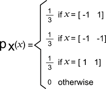
The support of X1 is described as follows: RX1 = {-1, 1} The probability mass function of X1 is shown below: 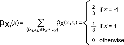
The expected value of X1 is shown below: 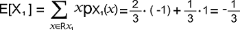
The expected value of X12 is shown below: 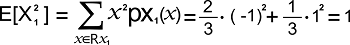
The variance of X1 is shown below: Var[X1] = E[X12] - E[X1]2 = 1 - (-1/3)2 = 8/9 The standard deviation of X1 is shown below: 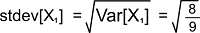
Now we will explain X2. The support of X2 is described as follows: RX2 = {-1, 1} And probability mass function of X2 is shown below: 
The expected value of X2 is shown below: 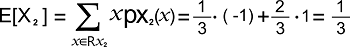
The expected value of X22 is shown below: 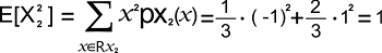
The variance of X2 is shown below: Var[X2] = E[X22] - E[X2]2 = 1 - (1/3)2 = 8/9 The standard deviation of X2 is shown below: 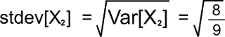
The expected value of X1X2 can be computed with the help of Transformation theorem, which is described as follows: 
Hence, the covariance between X1 and X2 is described as follows: Cov[X1, X2] = E[X1 X2] - E[X1] E[X2] = 1/3 - (-1/3) * 1/3 = 4/9 The linear correlation coefficient is described as follows: 
Correlation of Random variable with itselfIf there is a random variable X, then it will contain the following property: Corr[X, X] = 1 Proof: We can prove this in the following way: 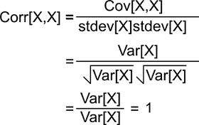
While proving this, we have used a fact that is described as follows: Cov[X, X] = Var[X] SymmetryThe linear correlation coefficient must be symmetric like this: Corr[X, Y] = Corr[Y, X] Proof: We can prove this in the following way: 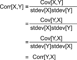
While proving this, we have use a fact covariance is symmetric, which is described as follows: Cov[X, Y] = Cov[Y, X] Examples of Linear correlation coefficientThere are various examples of the linear correlation coefficient, and some of them are described as follows: Example 1: In this example, we have a 2*1 discrete random vector which is denoted by X. The components of this vector are X1 and X2. Now we will assume that the support of X is: 
Its joint probability mass function is described as follows: 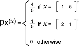
Here we have to calculate the coefficient of linear correlation between the components X1 and X2. Solution: The support of X1 is described as follows: RX1 = {1, 2} Its marginal probability mass function is described as follows: 
The expected value of X1 is described as follows: 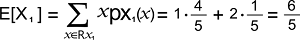
The expected value of X12 is described as follows: 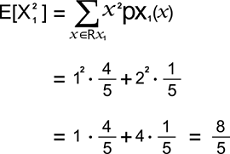
The variance of X1 is described as follows: Var[X1] = E[X12] - [X1]2 = 8/5 - (6/5)2 = (40-36)/25 = 4/25 The standard deviation of X1 is described as follows: 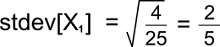
Now we will show the X2. So the support of X2 is described as follows: Rx2 = {1, 5} Its marginal probability mass function is described as follows: 
The expected value of X2 is described as follows: 
The expected value of X22 is described as follows: 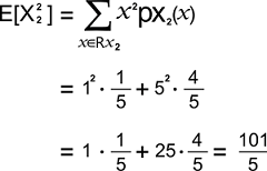
The variance of X2 is described as follows: Var[X2] = E[X22] - [X2]2 = 101/5 - (21/5)2 = (505-441)/25 = 64/25 The standard deviation of X1 is described as follows: 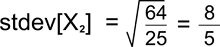
The expected value of X1X2 can be computed with the help of Transformation theorem like this: 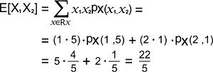
Hence, the covariance between X1 and X2 is described as follows: Cov[X1, X2] = E[X1 X2] - E[X1] E[X2] = 22/5 - (6/5) * 21/5 = (110-126)/25 = -16/25 The coefficient of linear correlation between X1 and X2 is described as follows: 
Example 2: In this example, we have a 2*1 discrete random vector, which is denoted by X. The entries of X are X1 and X2. Now we will assume that the support of X is: 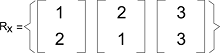
Its joint probability mass function is described as follows: 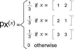
Here we have to calculate the coefficient of linear correlation between the entries X1 and X2. Solution: The support of X1 is described as follows: RX1 = {1, 2, 3} Its marginal probability mass function is described as follows: 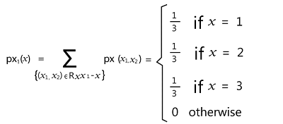
The mean of X1 is described as follows: 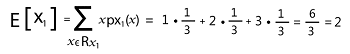
The expected value of X12 is described as follows: 
The variance of X1 is described as follows: Var[X1] = E[X12] - [X1]2 = 14/3 - (2)2 = (14-12) /3 = 2/3 The standard deviation of X1 is described as follows: 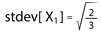
Now we will show X2. The support of X2 is described as follows: RX2 = {1, 2, 3} Its probability mass function is described as follows: 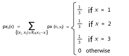
The mean of X2 is described as follows: 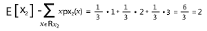
The expected value of X22 is described as follows: 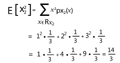
The variance of X2 is described as follows: Var[X2] = E[X22] - [X2]2 = 14/3 - (2)2 = (14-12) /3 = 2/3 The standard deviation of X2 is described as follows: 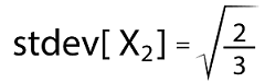
The expected value of X1X2 can be computed with the help of Transformation theorem like this: 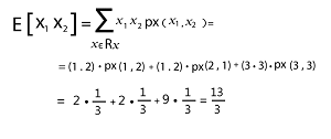
Hence, the covariance between X1 and X2 will become as follows when we put these pieces together: Cov[X1, X2] = E[X1 X2] - E[X1] E[X2] = 13/3 - 2 * 2 = (13-12) /3 = 1/3 The coefficient of linear correlation between X1 and X2 is described as follows: 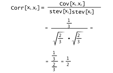
Example 3: In this example, we have a continuous random vector [X, Y], and we will assume that the support of this vector is: RXY = [0, ∞) * [1, 2] Its joint probability density function is described as follows: 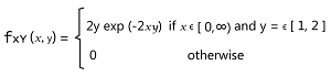
Here we have to calculate the coefficient of linear correlation between X and Y. Solution: The support of Y is described as follows: RY = [1, 2] The marginal probability density function of Y will be zero when there is a case y ? RY. We can get the marginal probability density function of Y with the help of integrating x out of the joint probability density in the following way: 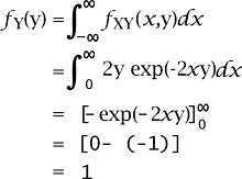
Thus, we can get the marginal probability density function of Y in the following way: 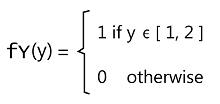
The expected value of Y is described as follows: 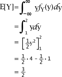
The expected value of Y2 is described as follows: 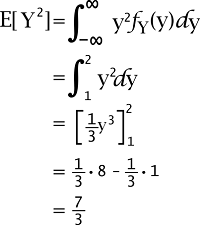
The variance of Y is described as follows: Var[Y] = E[Y2] - E[Y]2 = 7/3 - (3/2)2 = (28-27) /12 = 1/12 The standard deviation of Y is described as follows: 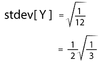
Now we will show X. The support of X is described as follows: Rx = [0, ∞) The marginal probability density function of X will be zero when there is a case x ? RX. We can get the marginal probability density function of X with the help of integrating y out of the joint probability density in the following way: 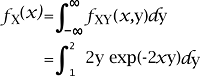
In this case, the integral cannot be explicitly computed for the density function but we can use the following way to write the marginal probability density function of X like this: 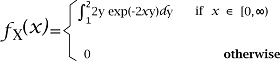
The expected value of X is described as follows: 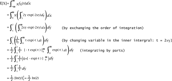
The expected value of X2 is described as follows: 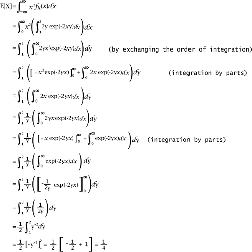
The variance of X is described as follows: Var[X] = E[X2] - E[X]2 = 1/4 - (1/2 In(2))2 = ¼ [1 - (In(2))2] = 1/12 The standard deviation of X is described as follows: 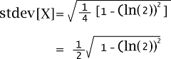
The expected value of XY can be calculated with the help of Transformation theorem like this, which is described as follows: 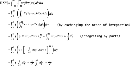
Hence, the covariance between X and Y will become as follows when we put these pieces together: Cov[X, Y] = E[XY] - E[X] E[Y] = 1/2 - 1/2 In(2) * 3/2 = 1/2 - 3/4 In(2) The coefficient of linear correlation between X and Yis described as follows: 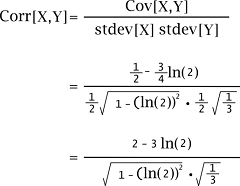
|
 .
. For Videos Join Our Youtube Channel: Join Now
Feedback
- Send your Feedback to [email protected]
Help Others, Please Share


