| |

Arima Model in PythonAn Introduction to Time Series ForecastingA Sequence of recording a metric over the constant time intervals is known as Time Series. Based on the frequency, a Time Series can be classified into the following categories:
Once we are done with Time Series Analysis, we have to forecast it in order to predict the future values that the series will be going to take. However, what is the need for forecasting? Since forecasting a Time Series, such as Sales and Demand, is often of incredible commercial value, which increases the need for forecasting. Time Series Forecasting is generally used in many manufacturing companies as it drives the primary business planning, procurement, and production activities. Any forecasts' errors will undulate throughout the chain of the supply or any business framework, for that stuff. Thus, it is significant in order to get accurate predictions saving the costs, and is critical to success. The Concepts and Techniques behind Time Series forecasting can also be applied in any business, including manufacturing. The Time Series forecasting can be broadly classified into two categories:
In the following tutorial, we will understand the specific type of method known as ARIMA modeling. Auto Regressive Integrated Moving Average, abbreviated as ARIMA, is an Algorithm for forecasting that is centered on the concept that the data in the previous values of the time series can alone be utilized in order to predict the future values. Let us understand the ARIMA Models in detail. An Introduction to ARIMA ModelsARIMA, abbreviated for 'Auto Regressive Integrated Moving Average', is a class of models that 'demonstrates' a given time series based on its previous values: its lags and the lagged errors in forecasting, so that equation can be utilized in order to forecast future values. We can model any Time Series that are non-seasons exhibiting patterns and not a random white noise with ARIMA models. There are three terms characterizing An ARIMA model: p, q, and d where,
If a Time Series has seasonal patterns, we have to insert seasonal periods, and it becomes SARIMA, short for 'Seasonal ARIMA'. Now, before understanding "the order of AR term", let us discuss 'd' term. What are 'p', 'q', and 'd' in the ARIMA model?The primary step is to make the time series stationary in order to build an ARIMA model. This is because the term 'Auto Regressive' in ARIMA implies a Linear Regression Model using its lags as predictors. And as we already know, Linear Regression Models work well for independent and non-correlated predictors. In order to make a series stationary, we will utilize the most common approach that is to subtract the past value from the present value. Sometimes, depending on the series complexity, multiple subtractions may be required. Therefore, the value of d is the minimum number of subtractions required to make the series stationary. And if the time series is already stationary, thus d becomes 0. Now, let us understand the terms 'p' and 'q'. The 'p' is the order of the 'AR' (Auto-Regressive) term, which means that the number of lags of Y to be utilized as predictors. At the same time, 'q' is the order of the 'MA' (Moving Average) term, which means that the number of lagged forecast errors should be used in the ARIMA Model. Now, let us understand what 'AR' and 'MA' models are in detail. Understanding Auto-Regressive (AR) and Moving Average (MA) ModelsIn the following section, we will discuss the AR and MA models and the actual mathematical formula for these models. A Pure AR (Auto-Regressive only) Model is a model which relies only on its own lags. Hence, we can also conclude that it is a function of the 'lags of Yt' 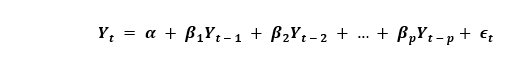
where, Yt-1 is the lag1 of the series. β1 is the coefficient of lag1 and is the term of intercept that is calculated by the model. Similarly, a Pure MA (Moving Average only) model is a model where Yt relies only on the lagged predicted errors. 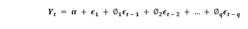
Where, the error terms are the AR models errors of the corresponding lags. The errors ϵt and ϵt-1 are the errors from the equations given below: 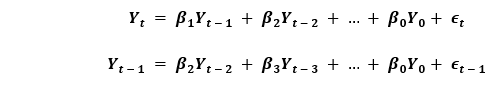
Thus, we have concluded Auto-Regressive (AR) and Moving Average (MA) models, respectively. Let us now understand the equation of an ARIMA Model. An ARIMA model is a model where the series of time was subtracted at least once in order to make it stationary, and we combine the Auto-Regressive (AR) and the Moving Average (MA) terms. Hence, we got the following equation: 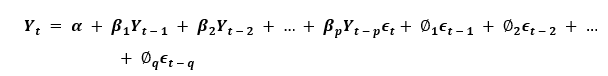
ARIMA Model in words: Forecasted Yt = Constant + Linear Combination Lags of Y (up to p lags) + Linear Combination of Lagged Predicted Errors (up to q lags) Thus, the objective of this model is to find the values of p, q, and d. However, how can we find one? Let us begin with finding the 'd' in the ARIMA Model. Finding the order of differencing 'd' in the ARIMA ModelThe primary purpose of differencing in the ARIMA model is to make the Time Series stationary. However, we have to take care of not over-differencing the series as an over-differenced series may also be stationary, which will affect the parameter of the model later. Now, let us understand the appropriate differencing order. The most appropriate differencing order is the minimum differencing needed in order to achieve an almost stationary series roaming around a defined mean and the ACF plat reaching Zero relatively faster. In case the autocorrelations are positive for multiple lags (generally, ten or more), the series requires further differencing. In contrast, if lag 1 autocorrelated itself pretty negatively, then the series is possibly over-differenced. In cases where we cannot actually decide between two differencing orders, then we have to choose the order providing the minor standard deviation in the differenced series. Let us consider an example to check if the series is stationary. We will use the Augmented Dickey-Fuller Test (adfuller()) from the statsmodels package of Python Programming Language. Example: Output: Augmented Dickey-Fuller Statistic: -2.464240 p-value: 0.124419 Explanation: In the above example, we have imported the adfuller module along with the numpy's log module and pandas. We have then used the pandas library to read the CSV file. We have then used the adfuller method and printed the values to the user. It is necessary to check whether the series is stationary or not. If not, we have to use difference; else, d becomes zero. The Augmented Dickey-Fuller (ADF) test's null hypothesis is that the time series is not stationary. Thus, if the ADF test's p-value is less than the significance level (0.05), then we will reject the null hypothesis and infer that the time series is definitely stationary. As we can observe, the p-value is more significant than the level of significance. Therefore, we can difference the series and check the plot of autocorrelation as shown below. Example: Output: 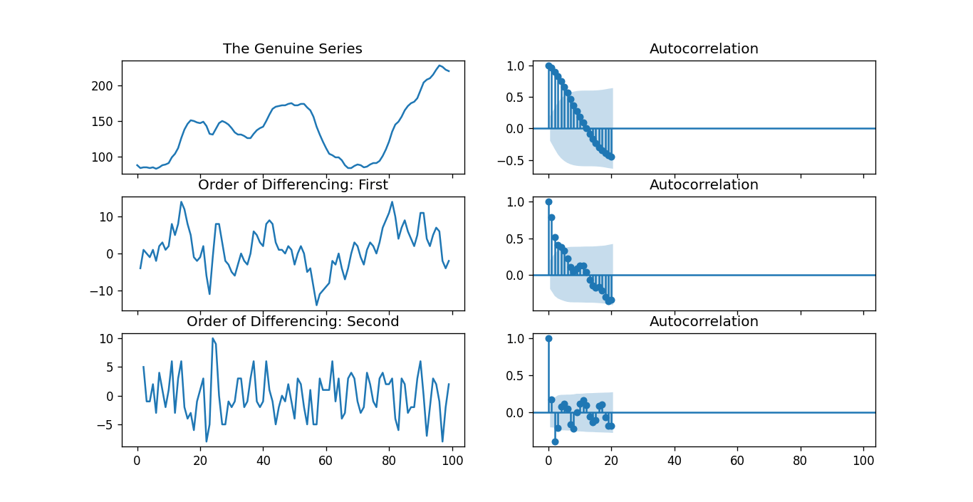
Explanation: In the above example, we have imported the required libraries and modules. We have then imported the data and plot different graphs. We have plotted the original series graph, first-order differencing, and second-order differencing along with their autocorrelation graphs. As we can observe, the time series has reached stationarity with two differencing orders. However, when we have a look at the plot of autocorrelation for the Second order of differencing, the lag going into the far negative zone pretty faster, indicating the series might have been over differenced. Hence, we will tentatively be fixing the differencing order because the series is not properly stationary, or we can say that the series has weak stationarity. This can be done as shown below. Example: Output: ADF Test = 2 KPSS Test = 0 PP Test = 2 Explanation: In the above example, we have imported the ndiffs method of the pmdarima module. We have then imported the dataset and defined 'X' as the object containing the values from the dataset. We used the ndiffs method to perform ADF, KPSS, and PP Tests and printed their results to the users. Finding the order of the Auto-Regressive (AR) term (p)In the following section, we will discuss the steps to check whether the model requires any Auto-Regressive (AR) terms. The number of AR terms needed can be found by studying the Partial Autocorrelation (PACF) plot. We can consider Partial Autocorrelation as the correlation between the series and its lag once we exclude the contributions from the intermediate lags. Thus, PACF tends to convey the pure correlation between the series and its lag. Hence, we can identify whether that lag is required in the Auto-Regressive (AR) term or not. Partial Autocorrelation of lag(k) of a series is the coefficient of that lag in the Auto-Regression Equation of Y. 
Now, let us understand how to find the number of AR terms? As we know, any Autocorrelation in a stationary series can be rectified by inserting enough AR terms. Thus, we can initially take the order of the Auto-Regressive (AR) term equivalent to as many lags that cross the limit of significance in the PACF Plot. Example: Output: 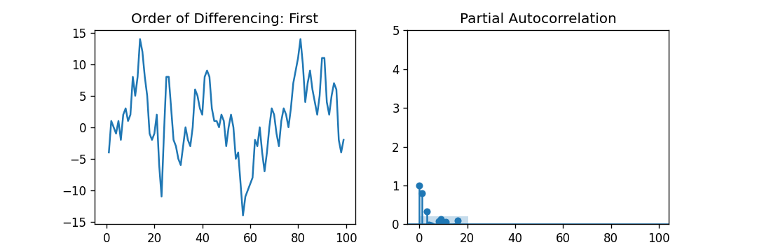
Explanation: In the above example, we have imported the required libraries, modules, and datasets. We have then plotted the graphs to represent the First Order Differencing and its partial autocorrelation. As a result, we can observe that the PACF lag 1 is pretty significant above the line of significance. Lag 2 also appears to be substantial, entirely maintaining to cross the limit of significance (blue region). However, we will be conservative and fix the p as one tentatively. Finding the Order of the Moving Average (MA) term (q)Similar to what we have looked at earlier at the PACF plot for the number of Auto-Regressive (AR) Terms, we can use the ACF plot to find the number of Moving Average (MA) Terms. A Moving Average (MA) term is, theoretically, the lagged forecast's error. The ACF plot expresses the number of Moving Average (MA) terms needed to remove the autocorrelation in the stationary series. Let us consider the following example to understanding the autocorrelation plot of the differenced series. Example: Output: 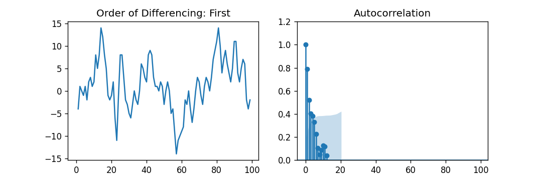
Explanation: In the above example, we have imported the required libraries, modules, and datasets. We have then plotted the graphs to represent the First Order Differencing and its Autocorrelation. As a result, we can observe that some lags are pretty above the line of significance. So, let us fix q as 2, tentatively. We can also use the simpler model in case of any doubt that adequately demonstrates the Y. Handling the A Slightly Under or Over-Differenced Time SeriesSometimes, a situation may occur where the series is slightly under-differenced, and differencing it one time extra makes the series somewhat over-differenced. In such cases, we have to add one or multiple additional Auto-Regressive (AR) Terms for the slightly under-differenced Time Series and add an extra Moving Average (MA) Term for the slightly over-differenced Time Series. Once we have discussed most of the topics, let us begin creating an ARIMA Model for Time Series Forecasting. Building the ARIMA ModelOnce we have determined the values of p, q, and d, we will try creating the ARIMA model. The implementation of the ARIMA() module is shown below: Example: Output:
ARIMA Model Results
==============================================================================
Dep. Variable:                D.value   No. Observations:                   99
Model:                 ARIMA(1, 1, 2)   Log Likelihood                -253.790
Method:                       css-mle   S.D. of innovations              3.119
Date:                Thu, 15 Apr 2021   AIC                            517.579
Time:                        21:10:37   BIC                            530.555
Sample:                             1   HQIC                           522.829

=================================================================================
                    coef    std err          z      P>|z|      [0.025      0.975]
---------------------------------------------------------------------------------
const             1.1202      1.290      0.868      0.385      -1.409       3.649
ar.L1.D.value     0.6351      0.257      2.469      0.014       0.131       1.139
ma.L1.D.value     0.5287      0.355      1.489      0.136      -0.167       1.224
ma.L2.D.value    -0.0010      0.321     -0.003      0.998      -0.631       0.629
                                    Roots
=============================================================================
                  Real          Imaginary           Modulus         Frequency
-----------------------------------------------------------------------------
AR.1            1.5746           +0.0000j            1.5746            0.0000
MA.1           -1.8850           +0.0000j            1.8850            0.5000
MA.2          545.5472           +0.0000j          545.5472            0.0000
-----------------------------------------------------------------------------
Explanation: In the above example, we have imported the new module called ARIMA from the statsmodels class and create the ARIMA model of the order 1, 1, and 2. We have then printed the summary of the model to the user. As we can observe, the overview of the model reveals a lot of details. The middle table is the table of coefficients where the 'coef' values act as the related terms' weights. We can also notice that the MA2 term's coefficient tends to zero, and the P-Value in the 'P > |z|' column is exceedingly insignificant. The P-Value should be less than 0.05, ideally for the corresponding X to be significant. Now, let us try rebuilding the model without the MA2 term. Example: Output:
ARIMA Model Results
==============================================================================
Dep. Variable:                D.value   No. Observations:                   99
Model:                 ARIMA(1, 1, 1)   Log Likelihood                -253.790
Method:                       css-mle   S.D. of innovations              3.119
Date:                Thu, 15 Apr 2021   AIC                            515.579
Time:                        21:34:00   BIC                            525.960
Sample:                             1   HQIC                           519.779

=================================================================================
                    coef    std err          z      P>|z|      [0.025      0.975]
---------------------------------------------------------------------------------
const             1.1205      1.286      0.871      0.384      -1.400       3.641
ar.L1.D.value     0.6344      0.087      7.317      0.000       0.464       0.804
ma.L1.D.value     0.5297      0.089      5.932      0.000       0.355       0.705
                                    Roots
=============================================================================
                  Real          Imaginary           Modulus         Frequency
-----------------------------------------------------------------------------
AR.1            1.5764           +0.0000j            1.5764            0.0000
MA.1           -1.8879           +0.0000j            1.8879            0.5000
-----------------------------------------------------------------------------
Explanation: In the above example, we have reduced the AIC of the model, which is actually good. We can also observe that the AR1 and MA1 terms' P-Values' have been improved and are highly significant (<< 0.05). Now, let us plot the residuals in order to ensure that there are no patterns such as constant mean and variance. Example: Output: 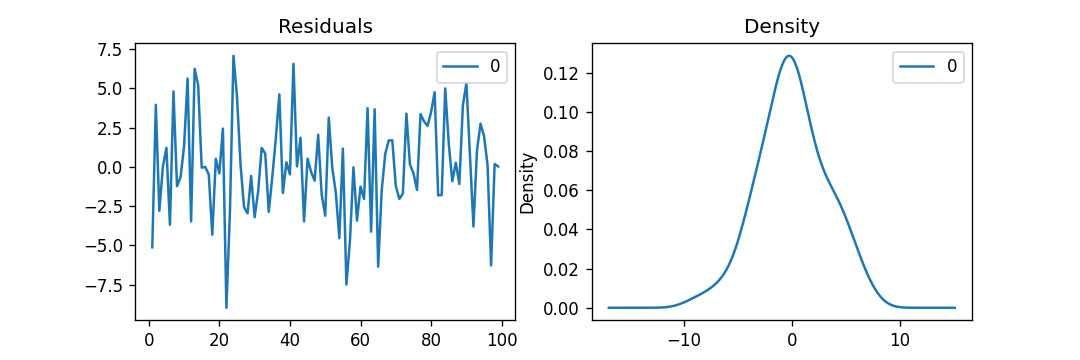
Explanation: In the above example, we have plotted the residual errors and density graphs. We can observe that the residual errors look fair with around zero mean and uniform variance. Let us plot the graph representing the actuals vs. fitted values with the help of the plot_predict() function. Example: Output: 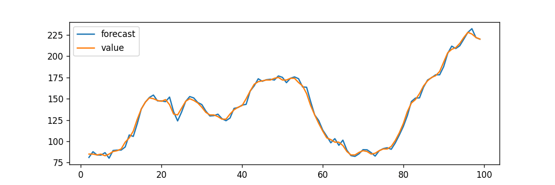
Explanation: In the above example, we have now plotted the 'actuals vs fitted' graph and set dynamic = False. As a result, the in-sample lagged values are utilized for forecasting. Thus, the model gets trained up until the past value makes the following forecast. Therefore, it can create the fitted forecast, and actuals appear preciously delicate.
Next TopicPython Modulus Operator
|
 For Videos Join Our Youtube Channel: Join Now
Feedback
- Send your Feedback to [email protected]
Help Others, Please Share


