| |

Solve Physics Computational Problems Using PythonThis article shows how to utilize Python to settle straightforward Laplace conditions with the Numpy library and Matplotlib to plot the arrangement of the situation. We'll likewise see that we can compose less code and accomplish more with Python. Presentation Laplace condition is a straightforward second-request incomplete differential condition. It is likewise a most straightforward illustration of elliptic incomplete differential condition. This condition is vital in science, particularly in physical science, since it portrays the conduct of electric and attraction potential and heat conduction. In thermodynamics (heat conduction), we call the Laplace condition a consistent state heat or intensity conduction condition. In this article, we will tackle the Laplace condition utilizing mathematical methodology as opposed to scientific/analytics approach. At the point when we say mathematical methodology, we allude to discretization. Discretization is a cycle to "change" the constant type of differential condition into a discrete type of differential condition; it likewise intends that with discretization, we can change the math issue into lattice polynomial math issue, which is inclined toward programming. Here, we must take care of a basic intensity conduction issue utilizing a limited contrast strategy. We will utilize Python Programming Language, Numpy (mathematical library for Python), and Matplotlib (library for plotting and envisioning information utilizing Python) as the apparatuses. We'll likewise see that we can compose less code and accomplish more with Python. BackgroundIn computational physical science, we "consistently" use programming to tackle the issue since PC programs can ascertain huge and complex estimations "rapidly". Computational physical science can be addressed in this graph. 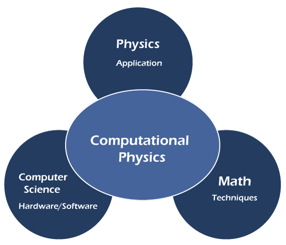
Many programming dialects are utilized today to tackle numerous mathematical issues, such as Matlab. In any case, here, we will utilize Python, the "simple to pick up" programming language, and obviously, it's free. It additionally has strong mathematical, logical, and information perception libraries like Numpy, Scipy, and Matplotlib. Python likewise gives equal execution, and we can run it in PC groups. Back to the Laplace condition, we will settle a straightforward 2-D intensity conduction issue involving Python in the following segment. Here, I expect the perusers have essential information on the limited contrast technique, so I don't compose the subtleties behind limited distinction strategy, subtleties of discretization blunder, dependability, consistency, combination, and quickest/ideal emphasizing calculation. We will skirt many strides of the computational equation here. Rather than tackling the issue with mathematical, logical approval, we show how to take care of the issue utilizing Python, Numpy, and Matplotlib, and, with a smidgen of the oversimplified feeling of computational physical science, so the source code here seems OK to general perusers who don't have practical experience in computational physical science. Challenges in Computational Physical ScienceComputational material science issues are overall undeniably challenging to settle precisely. This is because of a few (numerical) reasons: absence of logarithmic or potentially logical feasibility, intricacy, and tumult. For instance, - even clearly basic issues, for example, working out the wavefunction of an electron circling a particle in a solid electric field (Distinct impact), may require extraordinary work to plan a functional calculation (on the off chance that one can be found); other cruder or savage power procedures, for example, graphical strategies or root finding, might be required. On the further developed side, the numerical bother hypothesis is likewise some of the time utilized (a working is displayed for this specific model here). Moreover, the computational expense and intricacy for the overwhelming majority of body issues (and their traditional partners) will often develop rapidly. A visible framework commonly has a size of the request for {\displaystyle 10^{23}}10^{23} constituent particles, so it is generally an issue. Taking care of quantum mechanical issues is by and large of dramatic request in the system size [5], and for traditional N-body, it is of request N-squared. At long last, numerous actual frameworks are innately nonlinear, best-case scenario, and even from a pessimistic standpoint, turbulent: this implies it tends to be challenging to guarantee any mathematical mistakes don't develop with the result of delivering the 'arrangement' useless. Techniques and CalculationsSince computational material science utilizes a wide class of issues, it is partitioned among the different numerical issues it mathematically settles or the techniques it applies. Between them, one can consider:
Many strategies (and a few others) are utilized to compute the actual properties of the displayed frameworks. Computational material science likewise gets various thoughts from computational science. For instance, the thickness practical hypothesis utilized by computational strong state physicists to work out the properties of solids is fundamentally equivalent to that of scientific experts to ascertain the properties of particles. Moreover, computational material science envelops the product/equipment construction tuning to tackle the issues (as the issues normally can be exceptionally enormous in handling power needs or memory demands). PreparationsTo produce the result below, I use this environment:
In the event that you are running Ubuntu, you can utilize pip to introduce Numpy and Matplotib, or you can run this order in your Terminal. and use this command to install Matplotlib: Note that Python is, as of now, introduced in Ubuntu 14.04. To attempt Python, type Python in your Terminal and press Enter. You can likewise utilize Python, Numpy, and Matplotlib in Windows operating system, yet I like to utilize Ubuntu. Using the FormulaThis is the Laplace condition in 2-D cartesian directions (for heat condition): 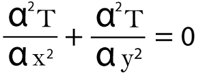
Where T is temperature, x will be x-aspect, and y will be y-aspect. x and y are elements of position in Cartesian directions. Assuming you are intrigued to see the scientific arrangement of the situation above, you can find it here. Here, we have to tackle the 2-D type of the Laplace condition. The issue to address is displayed underneath: 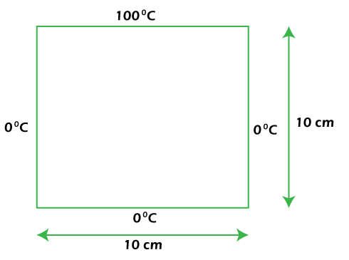
We will track down the consistent state temperature inside the 2-D plat (which likewise implies the arrangement of Laplace condition) above with the given limit conditions (temperature of the edge of the plat). Then, we will discretize the locale of the plat and gap it into meshgrid, and afterward, we will discretize the Laplace condition above with a limited distinction strategy. This is the discretized locale of the plat. 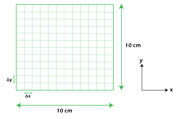
We set Δx = Δy = 1 cm and then make the grid as shown below: 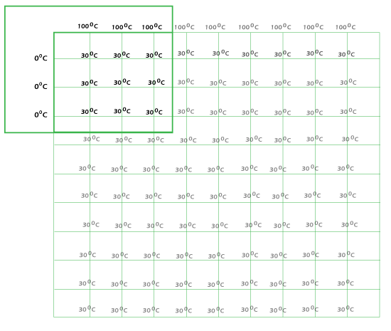
Note that the green hubs are our desired hubs to know the temperature (the arrangement), and the white hubs are the limit conditions (known temperature). Here is the discrete type of Laplace Condition above. 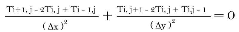
For our situation, the last discrete condition is displayed beneath. 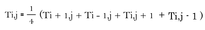
Presently, we are prepared to address the condition above. To address this, we use "surmise esteem" of inside lattice (green hubs); here, we set it to 30 degrees Celsius (or we can set it to 35 or other worth) since we don't have the foggiest idea about the worth inside the framework (obviously, those are our desired qualities to be aware). Then, we will repeat the condition until the distinction between esteem before cycle and the worth until emphasis is "Adequately little"; we call it combination. During the time spent emphasizing, the temperature esteem in the inside matrix will change itself; it's "self-correcting", so when we set supposition esteem nearer to its genuine arrangement, the quicker we get the "real" arrangement. 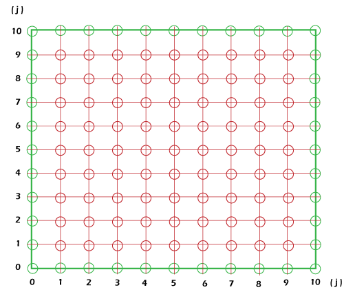
Step 1: We are prepared for the source code. To utilize the Numpy library, we want to import Numpy in our source code and also need to import Matplolib. Pyplot module to plot our answer. So, the initial step is to import fundamental modules. Code snippet: Step 2: Afterward, we set the underlying factors into our Python source code. Code snippet: Step 3: What we will do next is to set the "plot window" and meshgrid. Here is the code. Code snippet: Step 4: nps.meshgrid() makes the lattice network for us (we utilize this to plot the arrangement), the primary boundary is for the x-aspect, and the subsequent boundary is for the y-aspect. We use nps.arange() to organize a 1-D cluster with component esteem that beginnings from worth to some esteem; for our situation, it's from 0 to lenXs and from 0 to lenYs. Then we set the area: we characterize the 2-D cluster, characterize the size and fill the exhibit with surmise esteem; then, we put down the limit condition and take a gander at the language structure of filling the exhibit component for the limit condition above here. Code snippet: Step 5: Then, we are prepared to apply our last condition to the Python code beneath. We repeat the condition utilizing for circle. Code snippet: Step 6: You ought to know about the space of the code above; Python doesn't utilize sections, yet it utilizes blank areas or space. Indeed, the fundamental rationale is done. Then, we compose code to plot the arrangement, utilizing Matplotlib. Code snippet: Final Complete Source code.It's short, huh? OK, you can duplicate glue and save the source code, name it findif.py. To execute the Python source code, open your Terminal, and go to the index where you find the source code, type: furthermore, press Enter. Then the plot window will show up. Output: 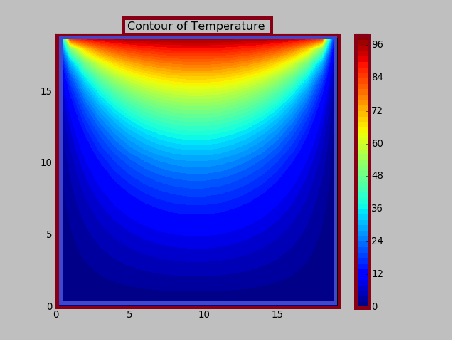
You can attempt to change the limit condition's worth; for instance, if you change the worth of the right edge temperature to 30 degrees Celcius (Trights = 30), then the outcome will seem to be this: 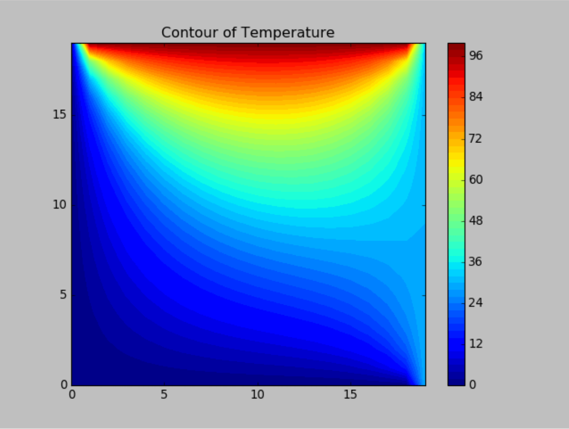
SummaryPython is a "simple to learn" and progressively composed programming language, and it gives (open source) a strong library for computational physical science or another logical discipline. Since Python is a deciphered language, it's delayed when contrasted with accumulated dialects like C or C++; however, it's not difficult to learn once more. We can likewise compose less code and accomplish more with Python, so we don't battle to program and zero in on what we need to address. In computational physical science, with Numpy and Scipy (numeric and logical library for Python), we can take care of numerous mind-boggling issues since it gives framework solver (eigenvalue and eigenvector solver), straight variable-based math activity, as well as sign handling, Fourier change, measurements, improvement, and so on. Notwithstanding its computational physical science, Python is additionally utilized in AI, even Google's TensorFlow purposes Python.
Next TopicScreen Rotation GUI Using Python Tkinter
|
 For Videos Join Our Youtube Channel: Join Now
Feedback
- Send your Feedback to [email protected]
Help Others, Please Share


