Project in Python - Breast Cancer Classification with Deep Learning

A malignant condition known as breast cancer is brought on by the unchecked growth of cells in the breast. Early treatment and diagnosis have been made possible by advancements in diagnosis and prevention. Women and men should be aware of the following symptoms and signs: a new lump or mass, nipple retraction, nipple or breast pain, redness, thickening of the nipple, scaliness of breast skin, or a nipple discharge (other than breast milk)

A biopsy is usually ordered when a doctor suspects breast cancer. A small amount of breast tissue is taken out under a microscope during the examination and procedure. Doctors classify each breast cancer case according to standard parameters like the disease's type, stage, grade, and gene expression to provide the most effective treatment. The cancer care medical team will determine a prognosis and treatment plan following confirmation of the diagnosis.

Based on Breast Cancer Types Classification

When tissue is examined during a biopsy, it can be determined whether there is cancer, adenocarcinoma, or another form, such as sarcoma.

The location and severity of the disease are typically used to classify cancer types.

Ductal carcinoma is the most prevalent, meaning that the illness first developed inside the ducts (pipes) carrying the milk toward the nipple. If cancer has not spread outside the duct and is categorized as in situ (DCIS), it is not invasive and therefore is contained within the duct; otherwise, it is described as metastatic breast cancer.

Other subtypes include triple-negative, inflammatory prostate, advanced breast cancer, and other uncommon breast cancer types.

Based on Breast Cancer Grades Classification

The disease is graded by pathologists as well. The grade is determined by how the tissue on the biopsy appears, how similar it appears to healthy cells, and how quickly the cancer cells divide. A lower grade typically denotes a slower rate of growth and a reduced risk of metastasis, whereas a higher grade denotes a faster rate of growth and a higher risk of spreading.

The Bloom-Richardson degree, Nottinghamshire grade, Device can grade, or Appeals to young grade can all be used to describe the histologic tumor grade. Grade 1 denotes well differentiation (closely resembling normal cells), while grade 2 denotes moderate differentiation. Poorly differentiating breast cancer is classified as grade 6. (almost unrecognizable and fast-growing.)

Breast Cancer Based on Genes Expression Classification

The American Cancer Society claims epigenetics is an additional and relatively new method for classifying breast cancer. Gene expression classifies breast tumors into four groups based on the PAM50 test's determination of their molecular characteristics.

Breast cancer types with luminal A and hydrophilic B gene expression patterns resemble tissue. Low-grade tumors with slow growth are Luminal A malignancies. Luminal B malignancies are more aggressive and have a higher rate of growth. When extra copies of the Target gene exist, HER2 breast cancer is identified.

The basal type, a member of the triple-negative types, is identified when there are normal levels but no detectable estrogen or progesterone receptors. The prevalence is higher in females who have the BRCA1 mutation. Basal cancer is more prevalent in younger and African-American women for unclear causes.

The website Breast Cancer News is solely focused on delivering news and details about the condition. It doesn't offer medical guidance, diagnosis, or care. This information does not replace qualified medical guidance, diagnosis, or care. Make sure to consider obtaining competent medical advice from what you have found on this website. Always ask your doctor or another knowledgeable health provider for advice if you have any concerns about a medical condition.

Learn the terminologies used in the Python Breast Cancer Classification project.

Deep Learning: What is it?

Deep Learning is a rigorous machine learning method that draws inspiration from the biological networks of neurons in the human brain. Convolutional neural networks, deep neural systems, perceptron, and deep belief networks are architectures that use numerous layers to pass data through before creating an output. Deep Learning is used in numerous domains, including computer vision, natural language processing, computational linguistics, audio recognition, and medication creation, to advance AI and enable many applications.

What is Keras?

Python-based Keras is a free neural network library. A greater API can be used with Theano, CNTK, and Python. The main goal of Keras is to provide quick experimentation and prototyping that works smoothly on CPU and GPU. It is expandable, modular, and user-friendly.

Breast Cancer Classification - About the Python Project

We'll create a classifier in this Python project to train on 80% of the breast cancer histopathological image dataset. We'll save 10% of the information for validation. We'll create a CNN (Artificial Neural Network), dubbed Cancernets, using Keras and train it using our image data. After that, we'll create a discriminant function to evaluate the model's effectiveness.

IDC, invasive ductal carcinoma, is the most prevalent type of breast cancer, accounting for 80% of all diagnoses. It begins in a milk duct and spreads to the fibrous or fatty cervix outside the channel. And the study of something like the microscopic structure underlying tissues is called histology.

The objective of Breast Cancer Classification

Constructing a Breast Prostate Cancer classifier using an IDC collection that can correctly identify a benign or malignant histological image.

The Dataset

We'll use Kaggle's IDC regular dataset, which contains breast cancer histology picture data. This dataset contains 2,77,52566 5050 patch images of prostate cancer tissues scanned at magnifications from 162 entire mount slide images. 1,98,768 of them suffer bad IDC tests, while 78,786 receive positive ones. The data set is openly accessible. 6.02Megabytes of disc space is required at the very least for this.

Prerequisites

You'll need to install a few Python packages to execute this sophisticated Python project. Use pip to accomplish this.

Approach for Advanced Project in Python - Breast Cancer Classification

Step 1: Get this zip file. Please arrive at the preferred location to unzip it.

Step 2: Now, create datasets in the directory for breast cancer classification; within this, create the original:

Step 3: Original 6 mkdir datasets mkdir datasets Make a copy of the dataset.

Step 4: The dataset can be unzipped in the original directory. We will use the tree command to examine this directory's structure:

Output:

((base) C: \Users\Sumeet Rathore\Desktop\breast-cancer-classification\breast-cancer-classification\datasets\original?tree
Folder PATH listing for volume windows
The volume serial number is 02FE-40C9
-10253
0
-1
-10254
-0
-1
-10255
�
1
-10256
-0
-1
-10257
-0
1
-10258
-0
-1
-10259
-0
1
-10260
-O

For each patient ID, we have a directory. We also have the 0 and 1 directories for images with benign and malignant content in each of these directories.

File name: config.py

We will require some configurations to construct the dataset and train the model. This can be found in the cancernets directory.

Explanation:

In this section, we specify the base path for the paths to the training, validation, and testing directories, the path to the input dataset (datasets/original), and the new directory (datasets/IDC). Additionally, we declare that training will consume 80% of the dataset, and validation will consume 10%.

File name: build_datasets.py

This will divide our dataset into training, validation, and testing sets according to the above ratio: 20% for testing and 10% for training. We will extract images in batches using the Keras ImageDataGenerator to avoid taking up memory space for the entire dataset at once.

Explanation:

Imports from shutil, imutils, config, random, and OS will be used in this. After a shuffle, we will compile a list of the original paths to the images. The length of this list is then multiplied by 0.8 to calculate an index, which enables us to slice it into sublists for the training and testing datasets. The remainder of the list is used for the training itself, with 10% of the list going to the training dataset for validation.

Now, a list of tuples containing information about the training, validation, and testing sets is called a dataset. For each, these hold the paths as well as the base path. We will print, for instance, "Building testing set" for each setType, path, and base path in this list. We will make the directory if there is no base path. Additionally, we will extract the class label and filename for each originalPaths path. We will construct the path to the label directory (0 or 1); if it does not already exist, we will explicitly create it. We will now construct the path to the final image and copy it where it belongs.

Step 5. Execute the build_datasets.py script

Output Screenshot:

C: \Users \ADMIN\Desktop\breast-cancer-classification\breast-cancer-classification>pybuild_dataset.py
Building training set
Building directory datasets/idc\training
Building directory datasets/idcltraining\e
Building directory datasets/ide\training\1
Building validation set
Building directory datasets/idclvalidation
Building directory datasets/idc\validation\1
Building directory datasets/idclvalidationle
Building testing set
Building directory datasets/idcltesting
Building directory datasets/idcltesting\1
Building directory datasets/idcltesting(0)

File name: cancernets.py

Cancernets will be the name of the network we build: a CNN (Convolutional Neural Network). This network carries out the following operations:

• Make use of three (6) CONV filters;
• Stack these filters on top of one another;
• carry out maximum pooling;
• employ depthwise separable convolution, which is more effective and uses less memory.

Quickly, the baseline model overfit. The model was made more consistent with both dropout placement settings.

As we can see, the model could not achieve higher training accuracy by placing the dropout layer after the pooling layer. TensorFlow employs element-wise dropout, in which the activation of some neurons is randomly masked by multiplying it by zero. Anyways, still, the same number of actual neurons are present. Therefore, applying a pooling operation to this is equivalent to applying a pooling operation to the output of the conv layer. On the other hand, when pooling is followed by dropout, we randomly remove some neurons from already reduced neurons. We have fewer neurons on which to train in this situation. Although we are not using the model's full potential in this situation, the regularization appears stronger.

The model with the dropout layer following the pooling layer had better generalizability. This is apparent from the test error rate.

There is no right or wrong way to use the dropout layer in the convolutional block. On the other hand, dropout after the pooling layer significantly reduces model capacity. For conv blocks, batch normalization is highly recommended. In the code section, we will figure out this.

Explanation:

Cancer news is constructed using the Sequential API, while depthwise convolutions are implemented using SeparableConv2D. The static method creates for the Cancernets class has four inputs: the image's width and height, its thickness (the number of color information in each image), as well as the number of classes the network will forecast between, which is 2 for us (0 and 1).

We initialize the models and shapes in this procedure. We modify the shape and the stream dimension when using channels first.

Three DEPTHWISE CONV = > RELU = > POOL layers will now be defined, each with a higher layering and more filters. The softmax classifier produces projection percentages for each class. Finally, we deliver the model.

As previously stated, batch normalization enables us to train our models at a faster learning rate, allowing our network to converge more quickly while avoiding internal covariate shifts.

This effect is demonstrated in this experiment. You won't believe how effective the straightforward concept of normalizing the input of hidden layers can be.

Observations The model with a learning rate of 0.01 trained without BN performed better when using Batch Normalization (BN) layers.

The non-BN model has 37,222 trainable parameters, while the BN-based model has 37,734. As a result, the number of trainable parameters increased only by 522, and those additional trainable parameters did not cause a significant change in the learning process. The point is that hidden representation normalization is effective.

The test error rate decreased to 29.1 percent with the same config of BN layers. This shows that BN is effective. For a 10-class classification model, the non-BN model's test error rate is 90%, which is random guessing.

As a result, we can speed up the training process and achieve faster convergence with appropriate learning rate scheduling using batch normalization.

Batch normalization, as previously discussed, enables us to train our models at a higher learning rate, allowing our network to converge more quickly while preventing internal covariate shifts.

This experiment demonstrates this outcome. You'll be astounded at how powerful the seemingly basic concept of normalizing the input of the convolution neurons can be.

Observations

With Batch Normalization (BN) layers, the deep learning algorithm without BN at a proportional gain of 0.01 outperformed the other models.

The BN-based model has 37,834 trainable parameters, compared to 37,322 for the non-BN model. Thus, the learning process stayed the same due to the 512 more trainable parameters that were included. The mandatory item to remember is that normalizing concealed forms works.

File name: train_models.py

This evaluates and trains the model. Let's import from numpy, keras, cancernets, sklearn, config, matplotlib, imutils, and os.

Explanation:

We begin this script by setting initial values for the batch size, learning rate, and the number of epochs. The number of training, validation, and testing paths in the three directories will be obtained. The class weight for the training data will then be obtained to correct the imbalance.

The training data augmentation object will now be initialized. Regularization is the process of making the models more general. We slightly modify the training examples here to avoid requiring additional training data. The validation and testing data augmentation objects will be initialized.

Now, we call fit.generator() to fit the model. The project dataset training, validation, and testing generators will be initialized to produce batches of images with the size batch_size. After that, we will use the Adagrad optimizer to initialize the models and use the binary_crossentropy loss function to compile them.

Our models have been successfully trained. Let's now evaluate the models using the test data. We will reset the generator and use the data to make predictions. The indices of the labels with the highest predicted probability for images from the testing set is then obtained. Additionally, a classification report will be shown.

Now that we have the raw accuracy, specificity, and sensitivity, we will compute the confusion matrix and display all the values. Last but not least, we'll plot the accuracy and training loss.

Output console screen:

WARNING: tensorflow: From C: \Users \ADMIN\ AppData \Local \Programs \Python \Python37 \lib\site-packages\tensorflow\python \ops \nn
 - - - - - - - - - - - - - - - - loved in a future version. - - - - - - - - - - - - - - - - - -
imp1.py: 180: add_dispatch_support.?locals>.wrapper (from tensorflow.python.ops.array_ops) is deprecated and will be rem
- - - - - - - - - - - - - - - - - Instructions for updating - - - - - - - - - - - - - - - - - -
Use tf. Wherein 2.0, which has the same broadcast rule as p.where
Epoch 1/40 6244/6244 [= 0.8370 = = = = ==] - 25905 415ms/step - loss: 0.3717 - acc: 0.8422 - val loss: 0.4139 - val acc: Epoch 2/40
6244/6244 [= 0.8471 I= = = = ==] - 24985 400ms/step - loss: 0.3464 - acc: 0.8527 - val loss: 0.3955 - val acc
Epoch 3/40 6244/6244 T = = = = ==] - 24805 397ms/step - loss: 0.3416 - acc: 0.8552 - val loss: 0.4203 - val acc:
? 0.8423 Epoch 4/40 6244/6244 [= = = = ==]
- 24985 400ms/step - loss: 0.3396 - aCC: 0.8562 - val loss: 0.4028 - val acc: 0.8414 Epoch 5/40 6244/ 6244 = = = = =] - 24395 391ms/step
- loss: 0.3388 - acc: 0.8573 - val loss: 0.3880 - val acc: 0.8461
- - - - - - - - - - - - - - - - - - Epoch 6/40 6244/6244 [= = = = ==]- - - - - - - - - - - - - - - - - -
- 24205 388ms/step - loss: 0.3366 - acc: 0.8573 - val loss: 0.3868 - val acc:
0.8460 Epoch 7/40 6244/6244===] - 24085 386ms/step - loss: 0.3363 - acc: 0.8578 - val loss: 0.3879 - val acc: 0.8456
Epoch 8/40 6244/6244= = = = =] - 24175 387ms/step - loss: 0.3355 - acc: 0.8580 - val loss: 0.3854 val acc: 565 6244/6244 [== 0.8529
Epoch 38/40 6244/6244 = = = = == 0.8513
Epoch 39/40 6244/ 6244 [ 0.8511 Epoch 40/40 6244/6244 [== 0.8516
- - - - - - - - - - - - - - - - - Now evaluating the model precision. - - - - - - - - - - - - - - - - - - 
OX = = = =] - 2382s 381ms/step - loss: 0.3303 - acc: 0.8605 - val loss: 0.3807 - val acc: ~ = = = =] - 2384s 382ms/step - loss: 0.3308
acc: 0.8599 - val loss: 0.3854 - val acc: = = = =] - 2676s 429ms/step - loss: 0.3317
acc: 0.8594 - val loss: 0.3847 - val acc: = = = =] - 23795 381ms/step loss: 0.3318
acc: 0.8598 - val loss: 0.3848 - val acc: recall
- - - - - - - - - - - - - - - - - - f1-score support- - - - - - - - - -- - - - - - - - - - 
C 30 0.91 0.72 0.87 0.79 0.89 0.75 39736 15769 accuracy macro ave
weighted ave 0.71 0.86 0.83 0.85 0.85 0.82 0.85 55505 557505 55505
?Data [[34757 4979] I 3271 12498]] Accuracy: 0.8513647419151428
Specificity: 0.79256769617579512626 Sensitivity: 0.8746980068451782
C: \Users \ADMIN\Desktop\breast-cancers-classifications\breast-cancer-classification>

The expected output graph looks like this: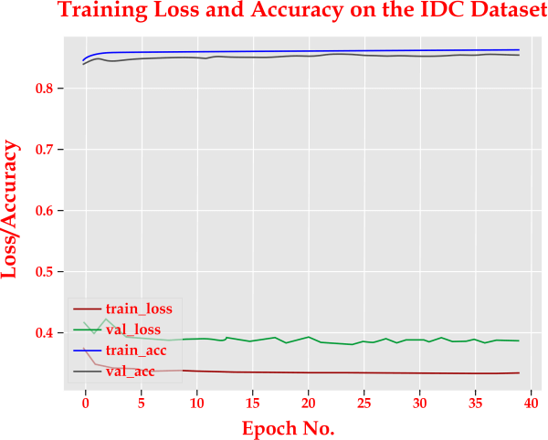

Summary

In this Python project, we developed the network Cancernets dataset and learned how to build a breast prostate cancer classifier using the IDC dataset (featuring histology images for Advanced Ductal Carcinoma). To do the same, we made advantage of keras library. I hope this Python project was enjoyable.