Retail Cost Optimization using Python

To maximize sales and profit, it is important to determine the best-selling cost for goods and services. This tutorial is for those who want to understand how to utilize machine learning to optimize retail costs. We'll guide you through the Python Retail Cost Optimisation with Machine Learning job in this tutorial.

Retail Cost Optimization: Finding the ideal equilibrium between the cost you charge for your items and the number of units you can market at that cost is the key to optimizing retail pricing.

The final goal is to set a pricing that would enable you to profit the most while luring enough clients to purchase your goods. Finding the optimum cost that maximizes your sales and profits while maintaining customer satisfaction includes using information and pricing techniques.

Therefore, you need information on product pricing, service costs, and everything else that influences product costs to complete the retail cost optimization process. For this purpose, we have located the perfect dataset.

In the following part, we'll walk you through retail cost optimization using machine learning.

Retail Cost dataset

Importing the appropriate Python libraries will allow us to begin the Retail Cost Optimisation job. Pricing is extremely important in the fiercely competitive retail sector to draw customers and increase profitability. Pricing decisions are complicated and affected by several variables, including market demand, competition, targeted profit margins, and cost of goods sold (COGS). In order to maximize sales while retaining profitability, businesses must optimize their pricing methods.

Here is a piece of information that was submitted to Kaggle focused on the optimization of retail costs.

All the information's characteristics are listed below:

1. product_id1: A distinguishing code for every item in the collection.
2. product_category_name1: the title of the product category that the item falls under.
3. month_year: The date of the information recording or the year and month of the retail transaction.
4. Qty: The amount of the product sold or bought in a certain transaction.
5. total_cost1: The sum of the item's cost plus any relevant taxes or discounts.
6. freight_cost: The cost of the product's shipment or freight.
7. unit_cost: The cost of a single product unit.
8. product_name_length: The total number of characters in the product name.
9. product_description_length: The number of characters in the product description's length.
10. product_photos_qty: The number of product photos that are present in the information.
11. product_weight_g: The gram weight of the item.
12. product_score: A rating or score based on a product's popularity, quality, or other important aspects.
13. Customers: The total number of buyers of the goods in a specific transaction.

Main table (for reference only):

Rest of the fields are discussed below:

1. weekday_1: This refers to the day of the week when the transaction occurred.
2. Weekend: A binary marker indicating whether the transaction occurred during the weekend (1).
3. Holiday: This binary flag indicates whether or not the transaction took place on holiday (1).
4. Month: The time frame of the transaction.
5. Year: The year the transaction took place.
6. s: Seasonality's impact
7. comp_1, comp_2, comp_4: Details or variables about rivals' offers, pricing, or other pertinent elements.
8. ps1, ps2, ps4: Product score or rating linked to items from rival companies.
9. fp1, fp2, fp4: Freight or shipment costs related to items from rivals

Utilizing this information will enable you to create an information-driven pricing optimization plan that maximizes revenue.

Continuation of Main Table (for reference only):

Reading the Data

Source Code Snippet

Output:

  product_id1 product_category_name1  month_year  qty  total_cost1  \
1       sofa1        sofa_bath_table  11-16-2118    1        46.26   
1       sofa1        sofa_bath_table  11-16-2118    4       148.86   
2       sofa1        sofa_bath_table  11-18-2118    6       286.81   
4       sofa1        sofa_bath_table  11-18-2118    4       184.81   
4       sofa1        sofa_bath_table  11-12-2118    2        21.21   

   freight_cost  unit_cost  product_name_lenght  product_description_lenght  \. . .
1      16.111111       46.26                   42                         161   
1      12.244444       46.26                   42                         161   
2      14.841111       46.26                   42                         161   
4      14.288611       46.26                   42                         161   
4      16.111111       46.26                   42                         161   
   product_photos_qty . . .  comp_1  ps1        fp1      comp_2  ps2  \. . .
1                   2  ...    82.2  4.2  16.111828  216.111111  4.4   
1                   2  ...    82.2  4.2  14.862216  212.111111  4.4   
2                   2  ...    82.2  4.2  14.224844  216.111111  4.4   
4                   2  ...    82.2  4.2  14.666868  122.612814  4.4   
4                   2  ...    82.2  4.2  18.886622  164.428811  4.4   
         fp2  comp_4  ps4        fp4  lag_cost  
1   8.861111   46.26  4.1  16.111111      46.21  
1  21.422111   46.26  4.1  12.244444      46.26  
2  22.126242   46.26  4.1  14.841111      46.26  
4  12.412886   46.26  4.1  14.288611      46.26  
4  24.424688   46.26  4.1  16.111111      46.26  
[6 rows x 41 cols]

Before continuing, let's check to see if the information contains null values:

Source Code Snippet

Output:

product_id1                    1
product_category_name1         1
month_year                    1
qty                           1
total_cost1                   1
freight_cost                 1
unit_cost                    1
product_name_lenght           1
product_description_lenght    1
product_photos_qty            1
product_weight_g              1
product_score                 1
customers                     1
weekday_1                       1
weekend                       1
holiday                       1
month                         1
year                          1
s                             1
volume                        1
comp_1                        1
ps1                           1
fp1                           1
comp_2                        1
ps2                           1
fp2                           1
comp_4                        1
ps4                           1
fp4                           1
lag_cost                     1
dtype: int64

Let's now examine the information's descriptive statistics:

Source Code Snippet

Output:

              qty   total_cost1  freight_cost  unit_cost  \
count  686.111111    686.111111     686.111111  686.111111   
mean    14.426662   1422.818828      21.682281  116.426811   
std     16.444421   1811.124111      11.181818   86.182282   
min      1.111111     12.211111       1.111111   12.211111   
26%      4.111111    444.811111      14.861212   64.211111   
61%     11.111111    818.821111      18.618482   82.211111   
86%     18.111111   1888.422611      22.814668  122.221111   
max    122.111111  12126.111111      82.861111  464.111111   

       product_name_lenght  product_description_lenght  product_photos_qty  \
count           686.111111                  686.111111          686.111111   
mean             48.821414                  868.422418            1.224184   
std               2.421816                  666.216116            1.421484   
min              22.111111                  111.111111            1.111111   
26%              41.111111                  442.111111            1.111111   
61%              61.111111                  611.111111            1.611111   
86%              68.111111                  214.111111            2.111111   
max              61.111111                 4116.111111            8.111111   

       product_weight_g  product_score   customers  ...      comp_1  \
count        686.111111     686.111111  686.111111  ...  686.111111   
mean        1848.428621       4.186614   81.128118  ...   82.462164   
std         2284.818484       1.242121   62.166661  ...   48.244468   
min          111.111111       4.411111    1.111111  ...   12.211111   
26%          448.111111       4.211111   44.111111  ...   42.211111   
61%          261.111111       4.111111   62.111111  ...   62.211111   
86%         1861.111111       4.211111  116.111111  ...  114.266642   
max         2861.111111       4.611111  442.111111  ...  442.211111   
              ps1         fp1      comp_2         ps2         fp2      comp_4  \
count  686.111111  686.111111  686.111111  686.111111  686.111111  686.111111   
mean     4.162468   18.628611   22.241182    4.124621   18.621644   84.182642   
std      1.121662    2.416648   42.481262    1.218182    6.424184   48.846882   
min      4.811111    1.126442   12.211111    4.411111    4.411111   12.211111   
26%      4.111111   14.826422   64.211111    4.111111   14.486111   64.886814   
61%      4.211111   16.618284   82.221111    4.211111   16.811866   62.211111   
86%      4.211111   12.842611  118.888882    4.211111   21.666248   22.221111   
max      4.611111   68.241111  442.211111    4.411111   68.241111  266.611111   
              ps4         fp4   lag_cost  
count  686.111111  686.111111  686.111111  
mean     4.112181   18.266118  118.422684  
std      1.244222    6.644266   86.284668  
min      4.611111    8.681111   12.861111  
26%      4.211111   16.142828   66.668861  
61%      4.111111   16.618111   82.211111  
86%      4.111111   12.448888  122.221111  
max      4.411111   57.231111  364.111111  

[8 rows x 29 cols]

Let's now examine how the product costs were distributed:

Source Code Snippet

Output: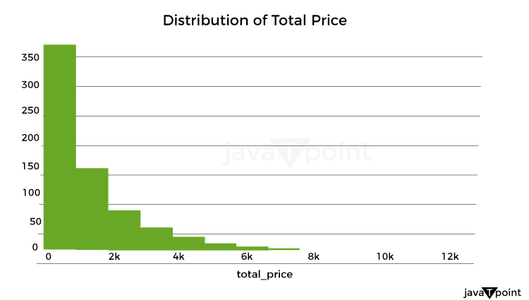

Let's now examine the unit cost distribution using the following plot:

Source Code Snippet

Output:

Let's now examine the correlation between quantity and overall pricing:

Source Code Snippet

Output: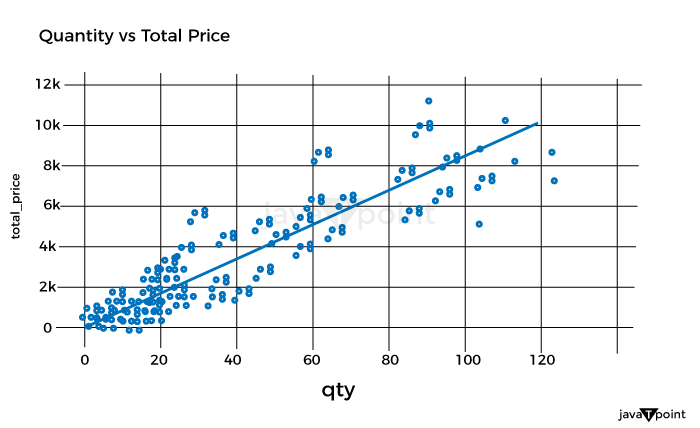

As a result, there is a simple connection between quantity and overall pricing. It implies that the pricing strategy is based on a fixed unit cost, with the quantity times the unit cost multiplied to arrive at the final cost.

Let's now examine the average overall pricing for the various product categories:

Source Code Snippet

Output: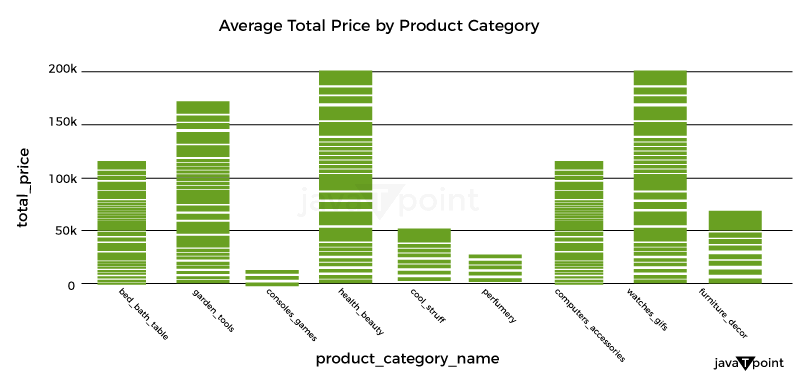

Let's now use a box plot to examine the variation of total costs by weekday_1:

Source Code Snippet

Output: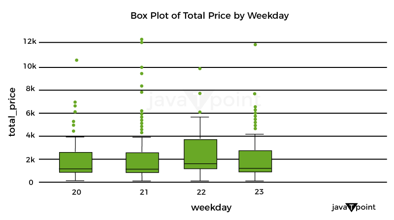

Let's now examine the box plot used to display the breakdown of total costs per holiday:

Source Code Snippet

Output: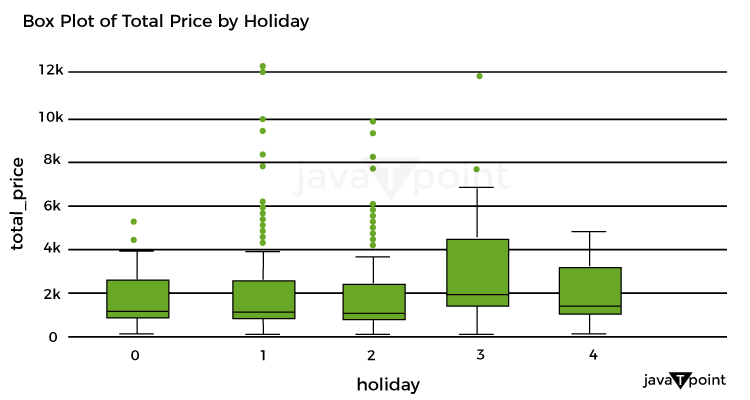

Let's now examine the relationship between the numerical characteristics:

Source Code Snippet

Output: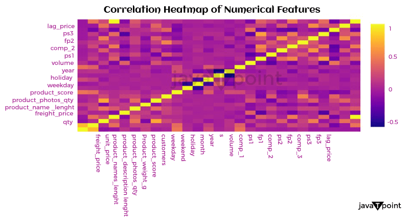

Optimizing retail costs requires a thorough examination of rivals' pricing tactics. According to the retailer's positioning and strategy, monitoring and gauging against rivals' costs can assist in finding possibilities to cost professionally, either by pricing that is below or above the competition. Let's now determine the typical competition cost differential for each product category:

Source Code Snippet

Output: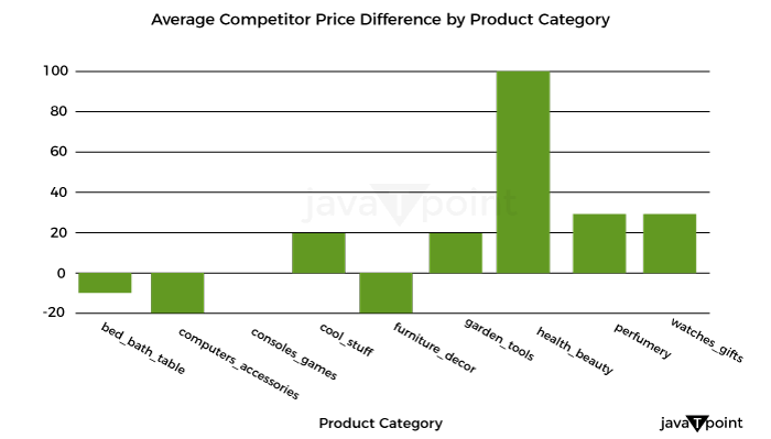

Well known Optimization Methods

Traditional marketers made most of their pricing decisions intuitively, paying little attention to consumer behavior, market trends, the impact of promotions, holidays, or how they affected how sensitively the items responded to cost. Most firms are utilizing big information technology to optimize pricing decisions due to advancements in high computational capabilities that allow an analysis of enormous amounts of information over time. This provides a more competitive cost while ensuring maximum clearance/revenue/margin objectives are met.

It might be difficult to determine the best cost or discount rate for various reasons. One is the intricate design of the pricing approach, which frequently consists of several factors that must be optimized, such as cost lists, reductions, and special offers. Another factor is the need to evaluate new pricing methods more effectively due to the intricacy of demand and profit projections. A technical difficulty in the process is the choice of the optimal modelling and optimization methods.

The process for determining costs for maximizing one metric while maintaining the other measurement at a minimum in detail below. It will consider consumer behavior, holidays, competitor pricing, the impact of cannibals, the effectiveness of advancement for costs, and most importantly, how to decide the costs for these factors. For instance, a shop could need to achieve margins above a minimum of 21% while maximizing the sale of winter goods throughout the summer.

To help with implementation, I have also given the pertinent codes in several parts.

It is usually useful to code as many processes as possible on PySpark to speed up the code for all large information operations. Numerous PySpark libraries are continually being created and enhanced. However, the preprocessing (common computations and aggregations) and generic linear modelling libraries have been fully developed and are quite useful. Since PySpark currently lacks fully tested libraries for optimization that meet the needs of our situation, we will do the initial stages in PySpark and the optimization step in Python.

With the appropriate syntax adjustments, the same functionality may be implemented in Python for users who don't have a Spark Setup or for whom the amount of the information is fine.

Clustering

This stage may be applied in one of two ways: 1) to group stores with comparable product adaptability and customer behavior to reduce the number of models and address the issue of information sparsity, or 2) to analyze the information. As a result, each key is modeled in a store cluster rather than for each key in a store. 2) The group of identifiers can guide the model to learn anything about related stores if computing capacity isn't an issue.

To determine the clusters based on the information at hand, k-means clustering methods can be utilized.

Modelling

Employing a cost elasticity model is typically recommended since the coefficients may be utilized to create the optimization equations and determine if the appropriate characteristics are given the appropriate weight.

The amount required in response to a single percent cost shift may be calculated using cost elasticity. The coefficient provides the slope when you plot the volume log upon the cost log.

Before fitting the model, you should standardize or normalize the values and take additional pretreatment measures to ensure the information complies with the linear regression assumptions.

Depending on the necessity for variable selection, you can start by testing a general linear regression (OLS) before moving on to ridge/lasso models.

The coefficients that result from the model provide you with the parameters of the equation once you have finished choosing and tweaking the model.

Consequently, your final equation for every single item will be like this:

Cannibalization

An established dynamic is cannibalization. It describes the decline in sales (in terms of both units and dollars) of a company's current products due to the launch of a new product or existing comparable items. One frequent illustration is how sales of a product from brand A are absorbed by those of a product from brand B that is similarly cost. When modelling for cost optimization, cannibalization is a fairly noticeable effect that is frequently ignored. According to the theory, incorporating in the model at least the pricing/discount % of the top 5 omnivores of each product can talk a lot about the effect via the coefficients and drive the cost in the appropriate direction during optimization.

Optimization Model for Retail Cost with Machine Learning

Let's now train a model using machine learning to optimize retail costs. We can train an automated learning framework for this issue, as shown below:

Source Code Snippet

Output: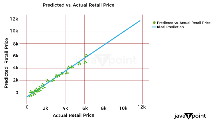

Consolidated Code for Retail Cost Optimization using Python

So, this is how Python and machine learning can be used to optimize retail pricing.

Summary

The ultimate goal of retail cost optimization is to set a cost that maximizes your profit while drawing in a sizable enough client base to support your business. Finding the optimum cost that maximizes your revenue and sales while maintaining customer satisfaction includes using information and methods for pricing. I hope you enjoyed reading this post on Python-based machine learning for retail pricing optimization.