| |
Python Tutorial
Python OOPs
Python MySQL
Python MongoDB
Python SQLite
Python Questions
Plotly
Python Tkinter (GUI)
Python Web Blocker
Python MCQ
Related Tutorials
Python Programs

Fourier Transform PythonIntroduction: In this article, we are briefly discussing Fourier Transform in Python. The mathematical remodel, referred to as a Fourier transform (feet), breaks features down into frequency components, represented by the rework's output as a function of frequency. Changes in time or area are the most not unusual kind, ensuing within the output of a feature based on either the temporal frequency or the spatial frequency, respectively. The evaluation is any other call for this method. Decomposing a musical chord's waveform in terms of its pitch intensity is one example of software. The mathematical characteristic that relates the frequency illustration to a space- or time-established domain is the "Fourier transform signal." The Fourier inversion theorem presents a way for synthesizing the authentic feature from its frequency area illustration. The remodel has a cost of zero for every frequency this is absent. The argument of the complex fee is the segment setting of that complex sinusoid. Maximum amplitude, peak-to-peak, RMS, and wavelength can all be used to describe the purple sinusoid. There may be a phase distinction among the pink and blue sinusoids. The Fourier transform is an effective tool for reading signals and is utilized in everything from audio processing to picture compression. SciPy offers a mature implementation within the scipy.fft module, and this article indicates a way to use it. The scipy.fft module may seem daunting at the start, as many features with often similar names and plenty of technical terms are used within the documentation without clarification. Happily, your handiest wants to apprehend a few key concepts to get started with modules. This algorithm plays a very important role in computing the Discrete Fourier Transform of a sequence. Convert spatial or temporal signals to frequency-domain signals. A DFT signal is created by distributing values into different frequency components. Converting the Fourier transform directly is computationally expensive. Therefore, the Fast Fourier Transform is used. This is because it is computed quickly by factoring the DFT matrix as a product of sparse coefficients. As a result, the DFT complexity is reduced from O(n2) to O(N log N). This makes a big difference when you are dealing with large datasets. Also, in direct comparison with the DFT definition, the FFT algorithm is very accurate in the presence of roundoff errors. This transform is from configuration to frequency space. It is very important in that it explores both transforms of a particular problem and the power spectrum of a signal for more efficient computation. This conversion can be from xn to xk. Transform spatial or temporal data into frequency domain data. Equation of the Fourier Transform: Equation of the Fourier transform is given below - 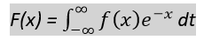
sympy.discrete.transforms.fft() function in python: It can perform Discrete Fourier transform (DFT) in complicated areas. Mechanically the series is padded with zero to the right because the radix-2 FFT requires the sample point quantity as an energy of two. For quick sequences, use this method with default arguments most effective as the complexity of expressions will increase with the dimensions of the collection. Parameters: Parameters of the above function are given below - seq: [repeatable] The sequence to apply the DFT. dps: [Integer] Number of decimal places of precision. Returns value: Returns value of the above function is given below - Fast Fourier Transform Example 1: Here, we give an example of sympy.discrete.transforms.fft() function in python. The example is given below - Output: Now we compile the above program, and after successful compilation, we run it. Then this result is visualizing - FFT : [84, -22.07107 + 39.04163*I, 20.0 - 10.0*I, -7.928932 + 9.041631*I, 16, -7.928932 - 9.041631*I, 20.0 + 10.0*I, -22.07107 - 39.04163*I] Example 2: Here, we give an example of sympy.discrete.transforms.fft() function in python. The example is given below - Output: Now we compile the above program, and after successful compilation, we run it. Then this result is visualizing - [33, -9 - 18*I, -11, -9 + 18*I] So, in this article we are briefly discussing Fourier transform in Python.
Next TopicIDLE Software in Python
|
 For Videos Join Our Youtube Channel: Join Now
Feedback
- Send your Feedback to [email protected]
Help Others, Please Share


