| |

Transfer Learning with Convolutional Neural NetworkArtificial neural networks (ANNs) are the most cutting-edge machine learning models in data science. Their performance is enigmatically astounding, and even with only one hidden layer, they can approximate any function with any desired level of precision. Why would anyone ever choose any other model given their amazing performance and widespread applicability? Before outperforming competing models, ANNs need a lot of data and computing power. Utilizing an ANN would be like using a spaceship for your daily commute for the datasets and technology people generally work with. So, one could ask, is there a method to benefit from ANNs without the disadvantages? Adaptive LearningTransfer learning is the process of using a model created for one purpose and applying it to another. Using the results of unsupervised machine learning, such as k-means clustering, as input in a supervised machine learning model, is a common example. Transfer learning can also be used to adapt a previously trained ANN to carry out a new task, which is the focus of this piece. We first need an overview of the fundamental structure of ANNs before we can talk about transfer learning with them. Fully Connected, Feed-Forward Neural Networks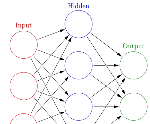
In its most basic form, an ANN is merely a set of layers of stacked logistic regressions, where each observation's feature value is represented by a node in the input layer, which is then multiplied by a weight and subjected to an activation function5 to inform each node of the subsequent layer (which is called a hidden layer). This procedure is repeated up to the output layer, which is the prediction. The forward propagation phase is this. The weights of each layer are then modified backwards when the predicted and actual values are compared to optimize some differentiable objective function. All the data and processing power are required during the learning phase of ANNs since each of the (millions of)6 weights must be adjusted using gradient descent on the loss function. That amounts to ten million calculus problems, challenging even for computers. In contrast, forward propagation simply multiplies values by weights, applies a straightforward activation function, and adds them. This is comparable to a few ten million math problems, which are easy for a machine to solve. Neural networks with convolutionsSpecialized ANNs called convolutional neural networks are employed for computer vision applications like object detection, object localization, and image categorization. Their design is identical to that of the straightforward ANN discussed above, with the exception that they start with a convolutional base intended to identify distinctive patterns in images. 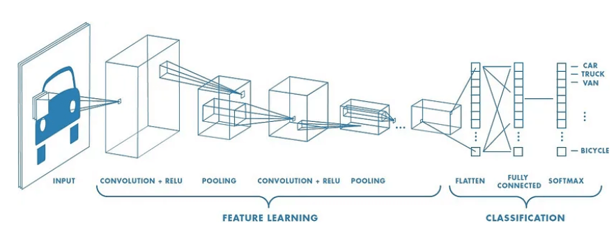
Convolutional layers that follow each other develop higher-order patterns (e.g., from edges to corners to shapes). The fully connected layers, which come after the convolutional base, learn the connections between these patterns and the labels, which serve as the foundation for their predictions. In only a few simple steps, we can adapt a sophisticated CNN that has been thoroughly trained for a broad goal, such as classification among a thousand different labels. First, the fully connected layers set up for the model's original function are removed, and they are then replaced with fully connected layers suitable for our particular goal (it is vital to note that the output layer's shape, activation function, and loss function may need to be modified). Then, we freeze the layers in the convolutional block so that, when the model is trained for our job, the pre-learned patterns are simply reinterpreted for the new context rather than being overwritten. And presto! Since only the fully connected layers need to be trained, we can do so with a small fraction of the data and processing power required to train the original model. Now we have a model with tens or hundreds of millions of learnt parameters ready to be fitted for our assignment. Even though performance would likely be better if the entire model were created from scratch for the the specific task, transfer learning is a handy little method for those without supercomputers or millions of tagged images.
Reusing the knowledge acquired from one activity for another is referred to as transfer learning. Many visual properties, specifically for convolutional neural networks (CNNs), are shared across several datasets (e.g. lines and edges are seen in almost every image). Because of this, particularly for huge constructions, Due to the lack of huge datasets and powerful computing resources, CNNs are rarely trained entirely from scratch. The 1.2 million-image ImageNet dataset is a typical pretraining set of images. The particular model used varies depending on the objective (often, users pick the model that does the best on the ImageNet challenge); however, this post uses the ResNet50 model. The pre-trained model is frequently accessible through the library used, in this example, Keras. Introduce ResNetThe vanishing gradient problem was the inspiration for the original design of ResNet. This issue restricts the size of a neural network since backpropagated gradients become incredibly small when multiplied repeatedly. By using skip connections-adding shortcuts that let data skip past layers-the ResNet architecture attempts to address this problem. A set of convolutional layers with skip connections, average pooling, and an output fully connected (dense) layer make up the model. When importing the model, we should exclude the convolutional layers as those are the only ones that contain the features we're interested in for transfer learning. Since we are removing them, the output layers must then be replaced with our layers. Problem StatementTo demonstrate the transfer learning process, I'll use the Caltech-101 image dataset with 101 categories and roughly 40-800 images per category. Processing of DataDownload the dataset first, then extract it. After extraction, be sure to delete the "BACKGROUND Google" folder. Code: We must divide the data into training and testing sets to evaluate accurately. To ensure proper representation in the test set, we must divide within each category. Output: 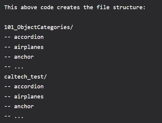
The train photographs are in the first folder, and the test images are in the second. The photos in each subfolder are organized by category. We'll employ Keras' ImageDataGenerator class to enter the data. ImageDataGenerator offers solutions for both augmentation and simple picture data processing. The code above builds an object for data created using the file path of the picture directory. Model Building Standard: Include the fundamental pretrained model. With most categories having under 50 image net, this dataset has only about 5628 images after splitting; therefore, fine-tuning the convolutional layers could lead to overfitting. Since our new and ImageNet datasets are comparable, we are certain that many pre-trained weights also use good features. So that they aren't altered while the rest of the classifier is trained, we can freeze those taught convolutional layers. Fine-tuning may still result in overfitting if you have a smaller dataset that differs significantly from the original dataset, but the later layers wouldn't have the right features. So that they aren't altered while the rest of the classifier is trained, we can freeze those taught convolutional layers. Fine-tuning may still result in overfitting if you have a smaller dataset that differs significantly from the original dataset, but the later layers wouldn't have the right features. Therefore, you could once more freeze the convolutional layers, but this time, just utilize the results from earlier layers since they have more generic features. You can frequently fine-tune the entire network with a large dataset without worrying about overfitting. We may now include the remaining classifier. As a result, a different classifier trained on the new dataset is fed the output from the previously taught convolutional layers. Model training code Output: 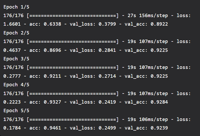
To evaluate the test set, use code. Output: 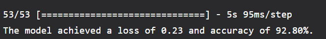
After only five epochs, we obtained 92.8% accuracy for a 101-class dataset. For context, the original ResNet was trained across 120 epochs on a dataset of about 1 million images. There are a few areas that could use improvement. The difference between validation loss and training loss in the most recent epoch indicates that the model is beginning to overfit. Image augmentation is one technique to address this. The ImageDataGenerator class makes it simple to implement simple picture augmentation. |
 For Videos Join Our Youtube Channel: Join Now
Feedback
- Send your Feedback to [email protected]
Help Others, Please Share


