Difference Between Prim's and Kruskal's algorithm

Introduction:

In the field of graph theory, finding the minimum spanning tree (MST) of a given graph is a common problem with numerous applications. MSTs are used in various fields, such as network design, clustering, and optimization. Two popular algorithms to solve this problem are Prim's and Kruskal's algorithms. While both algorithms aim to find the minimum spanning tree of a graph, they differ in their approaches and the underlying principles they rely on.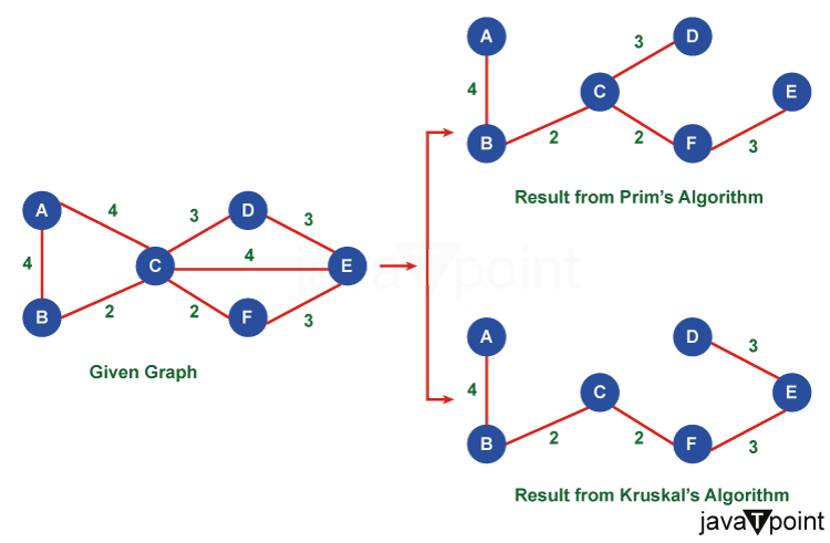

Difference Between Prim's and Kruskal's algorithm

Prim's Algorithm:

Prim's algorithm is a greedy algorithm that incrementally grows the minimum spanning tree from a starting vertex. The algorithm maintains two sets of vertices: one set contains the vertices already included in the MST, while the other set contains the remaining vertices. Prim's algorithm iteratively selects the vertex with the smallest edge weight that connects the two sets and adds it to the MST.

The algorithm follows the following steps:

Initialization: Choose a starting vertex and mark it as visited.
Find the minimum-weight edge connected to the visited vertices.

To accomplish this, examine all edges connected to the visited vertices and select the one with the lowest weight.

Select the edge with the lowest weight and add it to the MST.
Mark the newly added vertex as visited.
Repeat steps 2-4 until all vertices are visited.

Key Characteristics of Prim's Algorithm:

Prim's algorithm is a greedy approach, as it makes locally optimal choices at each step to construct the MST.

It guarantees the generation of a connected and acyclic MST.

The time complexity of Prim's algorithm is O(V^2) with a simple implementation using an adjacency matrix. However, using a priority queue can reduce the complexity to O(E log V).

Program

#include <iostream>
#include <vector>
#include <queue>
#include <climits>

using namespace std;

// Structure to represent a graph edge
struct Edge {
    int destination;
    int weight;
};

// Function to find the minimum spanning tree using Prim's algorithm
void primMST(vector<vector<Edge>>& graph, int startVertex) {
    int numVertices = graph.size();

    // Create a vector to store the key (minimum weight) of each vertex
    vector<int> key(numVertices, INT_MAX);

    // Create a vector to store the parent of each vertex in the minimum spanning tree
    vector<int> parent(numVertices, -1);

    // Create a vector to store whether a vertex is included in the minimum spanning tree
    vector<bool> included(numVertices, false);

    // Priority queue to store the vertices and their key values
    priority_queue<pair<int, int>, vector<pair<int, int>>, greater<pair<int, int>>> pq;

    // Start with the given startVertex
    pq.push(make_pair(0, startVertex));
    key[startVertex] = 0;

    while (!pq.empty()) {
        int u = pq.top().second;
        pq.pop();

        included[u] = true;

        // Traverse all adjacent vertices of u
        for (const auto& edge : graph[u]) {
            int v = edge.destination;
            int weight = edge.weight;

            // If v is not included in the minimum spanning tree
            // and the weight of the edge (u, v) is smaller than the current key of v
            if (!included[v] && weight < key[v]) {
                // Update the key of v
                key[v] = weight;
                parent[v] = u;
                pq.push(make_pair(key[v], v));
            }
        }
    }

    // Print the minimum spanning tree
    cout << "Minimum Spanning Tree:" << endl;
    for (int i = 1; i < numVertices; ++i) {
        cout << parent[i] << " - " << i << endl;
    }
}

int main() {
    int numVertices, numEdges;
    cout << "Enter the number of vertices: ";
    cin >> numVertices;
    cout << "Enter the number of edges: ";
    cin >> numEdges;

    vector<vector<Edge>> graph(numVertices);

    cout << "Enter the edges (source, destination, weight):" << endl;
    for (int i = 0; i < numEdges; ++i) {
        int source, destination, weight;
        cin >> source >> destination >> weight;

        Edge edge;
        edge.destination = destination;
        edge.weight = weight;

        graph[source].push_back(edge);
        // Uncomment the line below if the graph is undirected
        // graph[destination].push_back(edge);
    }

    int startVertex;
    cout << "Enter the start vertex: ";
    cin >> startVertex;

    primMST(graph, startVertex);

    return 0;
}

Explanation:

The main function begins by asking the user to input the number of vertices and edges in the graph.
It creates a 2D vector called graph to represent the adjacency list of the graph. The size of the vector is determined by the number of vertices.
The program then asks the user to input the edges of the graph one by one. For each edge, the user is prompted to enter the source vertex, destination vertex, and weight of the edge. The edge is added to the adjacency list of both the source and destination vertices.
The user is asked to enter the start vertex from which the minimum spanning tree will be constructed.
The primMST function is called with the graph and startVertex as arguments.
Inside the primMST function, the number of vertices is determined from the size of the graph vector.
Three vectors, key, parent, and included, are initialized. The key vector stores the minimum weight of each vertex, the parent vector stores the parent of each vertex in the MST, and the included vector keeps track of whether a vertex is already included in the MST.
A priority queue called pq is created to store pairs of vertices and their key values. The priority queue is implemented as a min-heap using the greater comparator, ensuring that the vertex with the smallest key value is at the top.
The start vertex is added to the priority queue with a key value of 0.
The program enters a loop that continues until the priority queue pq is empty.
In each iteration of the loop, the vertex with the minimum key value is extracted from the priority queue. This vertex is marked as included in the MST.
The program then iterates over all adjacent vertices of the extracted vertex. For each adjacent vertex that is not already included in the MST and has an edge weight smaller than its current key value, the key value is updated, the parent is set to the extracted vertex, and the vertex is added to the priority queue.
After the loop ends, the minimum spanning tree is printed by iterating over the parent array. Each entry in the parent array represents an edge in the MST, and the program prints the parent-child relationship for each vertex except the start vertex.

Program Output:

Kruskal's Algorithm:

Kruskal's algorithm is another greedy algorithm used to find the minimum spanning tree. Unlike Prim's algorithm, Kruskal's algorithm processes the edges of the graph in ascending order of their weights. It incrementally adds edges to the MST as long as they do not create a cycle.

The steps involved in Kruskal's algorithm are as follows:

Sort all the edges in non-decreasing order of their weights.
Initialize an empty graph as the MST.
Consider the edges in the sorted order and add them to the MST if they do not create a cycle.

To determine if adding an edge creates a cycle, Kruskal's algorithm utilizes the concept of disjoint sets. It keeps track of the subsets that contain each vertex and checks if adding an edge connects two vertices from the same subset.

Key Characteristics of Kruskal's Algorithm:

Kruskal's algorithm uses the concept of disjoint sets to detect cycles efficiently.

It does not require a starting vertex and is not restricted to a connected graph.

The time complexity of Kruskal's algorithm is O(E log E) or O(E log V) with efficient sorting algorithms, where E represents the number of edges and V the number of vertices.

Program

#include <iostream>
#include <vector>
#include <algorithm>

using namespace std;

// Structure to represent an edge
struct Edge {
    int source, destination, weight;
};

// Structure to represent a disjoint set
struct DisjointSet {
    vector<int> parent, rank;
};

// Create a disjoint set
DisjointSet createSet(int vertices) {
    DisjointSet ds;
    ds.parent.resize(vertices);
    ds.rank.resize(vertices);
    for (int i = 0; i < vertices; i++) {
        ds.parent[i] = i;
        ds.rank[i] = 0;
    }
    return ds;
}

// Find the set to which an element belongs
int find(DisjointSet &ds, int vertex) {
    if (vertex != ds.parent[vertex]) {
        ds.parent[vertex] = find(ds, ds.parent[vertex]);
    }
    return ds.parent[vertex];
}

// Union of two sets
void unionSets(DisjointSet &ds, int x, int y) {
    int xroot = find(ds, x);
    int yroot = find(ds, y);
    if (ds.rank[xroot] < ds.rank[yroot]) {
        ds.parent[xroot] = yroot;
    } else if (ds.rank[xroot] > ds.rank[yroot]) {
        ds.parent[yroot] = xroot;
    } else {
        ds.parent[yroot] = xroot;
        ds.rank[xroot]++;
    }
}

// Comparator function to sort edges by weight
bool compareEdges(const Edge &a, const Edge &b) {
    return a.weight < b.weight;
}

// Kruskal's algorithm to find minimum spanning tree
vector<Edge> kruskalMST(vector<Edge> &edges, int vertices) {
    vector<Edge> result;
    DisjointSet ds = createSet(vertices);

    sort(edges.begin(), edges.end(), compareEdges);

    for (const auto &edge : edges) {
        int x = find(ds, edge.source);
        int y = find(ds, edge.destination);

        if (x != y) {
            result.push_back(edge);
            unionSets(ds, x, y);
        }
    }

    return result;
}

// Utility function to print the minimum spanning tree
void printMST(vector<Edge> &mst) {
    cout << "Minimum Spanning Tree:" << endl;
    int totalWeight = 0;
    for (const auto &edge : mst) {
        cout << edge.source << " -- " << edge.destination << " : " << edge.weight << endl;
        totalWeight += edge.weight;
    }
    cout << "Total weight of the minimum spanning tree: " << totalWeight << endl;
}

// Main function
int main() {
    int vertices, edges;
    cout << "Enter the number of vertices in the graph: ";
    cin >> vertices;
    cout << "Enter the number of edges in the graph: ";
    cin >> edges;

    vector<Edge> graph(edges);

    cout << "Enter the details of each edge (source, destination, weight):" << endl;
    for (int i = 0; i < edges; i++) {
        cout << "Edge " << i + 1 << ": ";
        cin >> graph[i].source >> graph[i].destination >> graph[i].weight;
    }

    vector<Edge> minimumSpanningTree = kruskalMST(graph, vertices);
    printMST(minimumSpanningTree);

    return 0;
}

Explanation:

The DisjointSet struct has two vectors: parent and rank. The parent vector stores the parent of each vertex, and the rank vector is used to optimize the union operation in the disjoint set data structure.
The program then defines several helper functions. The createSet function initializes a disjoint set by assigning each vertex to its own set. The find function finds the set to which an element belongs using path compression.
The unionSets function performs the union of two sets by rank, ensuring that the smaller set is always merged into the larger set. The compareEdges function is a comparator used to sort the edges in non-decreasing order of their weights.
The kruskalMST function takes the vector of edges and the number of vertices as input and returns a vector of edges representing the minimum spanning tree.
It initializes an empty result vector and creates a disjoint set using the createSet The edges are then sorted in non-decreasing order of their weights using the sort function and the compareEdges comparator.
The program then iterates through each edge in the sorted order. For each edge, it finds the sets to which the source and destination vertices belong using the find function.
If the sets are different, indicating that the vertices are not already connected, the edge is added to the result vector, and the sets are merged using the unionSets
Finally, the printMST function is called to display the minimum spanning tree. It prints each edge in the MST along with its weight and calculates the total weight of the MST.
In the main function, the user is prompted to enter the number of vertices and edges in the graph. Then, the details of each edge (source, destination, and weight) are taken as input from the user.
The kruskalMST function is called with the input graph and vertices, and the resulting minimum spanning tree is printed using the printMST

Program Output:

Differences in Approach:

Approach:

Prim's algorithm uses a vertex-based approach, focusing on growing the MST from a starting vertex. It gradually expands the tree by adding the minimum-weight edges connected to the visited vertices.

Kruskal's algorithm uses an edge-based approach, sorting edges and adding them to the MST as long as they don't form a cycle. It constructs the MST by considering edges one by one in ascending order of their weights.

Connectivity:

Prim's algorithm ensures that the MST is always connected, even for disconnected input graphs. It starts with a single vertex and gradually expands the tree until it encompasses all vertices.

Kruskal's algorithm can generate multiple trees in the case of a disconnected graph. It treats each vertex as an individual tree initially and merges them as edges are added, resulting in a forest of trees.

Time Complexity:

Prim's algorithm has a time complexity of O(V^2) with a simple implementation and O(E log V) with a priority queue. The choice of implementation depends on the density of the graph.

Kruskal's algorithm has a time complexity of O(E log E) or O(E log V) with efficient sorting algorithms. It primarily depends on the number of edges rather than the number of vertices

Advantages of Prim's Algorithm:

Efficiency: Prim's algorithm performs well on dense graphs where the number of edges is close to the maximum possible. Its time complexity is O(V^2) with an adjacency matrix representation.

Guaranteed MST: Prim's algorithm guarantees that the MST is found within V-1 iterations, where V is the number of vertices in the graph.

Simplicity: Prim's algorithm is relatively easy to understand and implement, making it a popular choice for educational purposes.

Disadvantages of Prim's Algorithm:

Requirement of Connected Graphs: Prim's algorithm assumes a connected graph. If the graph has disconnected components, the algorithm needs to be applied to each component separately to find their respective minimum spanning trees.

Inability to Handle Negative Weights: Prim's algorithm cannot handle graphs with negative edge weights since it may lead to incorrect MST results.

Performance on Sparse Graphs: For sparse graphs with a significantly smaller number of edges, Prim's algorithm may be less efficient compared to Kruskal's algorithm.

Applications of Prim's Algorithm:

Network Design: Prim's algorithm is commonly used in network design scenarios to find the minimum cost network that connects various locations, minimizing the overall connection cost.

Cluster Analysis: It can be applied to identify clusters or communities in a network, where each cluster is represented by a subtree of the minimum spanning tree.

Advantages of Kruskal's Algorithm:

Handling Disconnected Graphs: Kruskal's algorithm naturally handles disconnected graphs and produces a minimum spanning forest, which consists of multiple MSTs for each connected component.

Handling Negative Weights (with No Negative Cycles): Kruskal's algorithm can handle graphs with negative edge weights, as long as there are no negative cycles present in the graph.

Efficiency for Sparse Graphs: Kruskal's algorithm performs better on sparse graphs, where the number of edges is significantly smaller. Its time complexity is O(E log E), where E is the number of edges.

Disadvantages of Kruskal's Algorithm:

Sorting Overhead: Kruskal's algorithm requires sorting the edges based on their weights, which introduces an additional O(E log E) time complexity.

Potential Forest Output: In the case of disconnected graphs, Kruskal's algorithm may produce a forest of multiple minimum spanning trees, which might not be desirable for some applications.

Applications of Kruskal's Algorithm:

Network Connectivity: Kruskal's algorithm is useful for determining whether a network is fully connected or not by finding the minimum spanning forest, which represents the connections between components.

Image Segmentation: It can be applied in image processing tasks to partition an image into distinct regions by treating pixels as vertices and the similarity between pixels as edge weights.

Next TopicInterpolation Search

← prev next →