Shortest distance between two cells in a matrix or grid

The problem of changing the shortest distance between two cells in a matrix or grid is a classic algorithmic challenge with operations in colorful fields such as robotics, navigation systems, and computer games.

Given a matrix or grid where each cell may represent a different state or handicap, the ideal is to determine the shortest path between two specified cells. Generally, the allowed movements are confined to the over, down, left, and right directions between conterminous cells.

One generally used algorithm to solve this problem is breadth-first search (BFS). BFS explores the grid position by position, starting from the source cell and marking visited cells until the destination cell is reached. The first time the destination cell is encountered, the algorithm terminates, and the distance is calculated.

Way for the BFS algorithm

Start with the source cell and enqueue it into a line.
While the line isn't empty, dequeue a cell and explore its neighbors.
Mark each visited cell to avoid spare disquisitions.
Continue this process until the destination cell is reached.
Calculate the distance from the source to the destination.

Enforcing BFS involves maintaining a line to manage the order of discourse and a visited array to track cells that have formerly been reused.

This algorithm efficiently guarantees the shortest distance between two cells in the matrix by methodically exploring the grid.

Algorithm.

The algorithm for chancing the shortest distance between two cells in a matrix or grid using breadth-first search (BFS) can be outlined as follows:

Initialize data structures.
Produce a line to keep track of cells to be explored.
Produce a 2D array (visited) to mark cells that have been visited to avoid spare disquisition.
Enqueue the Start Cell
Enqueue the starting cell into the line along with the 0 distance.
Mark the starting cell as visited.
BFS Exploration
While the line isn't empty
Dequeue a cell from the front of the line.
Explore its neighbors (over, down, left, right).
For each unvisited neighbor
Mark the neighbor as having visited.
Enqueue the neighbor into the line along with an incremented distance.
Destination Reached
Still, return the advised distance if the destination cell is reached during the discourse.
Destination unobtainable

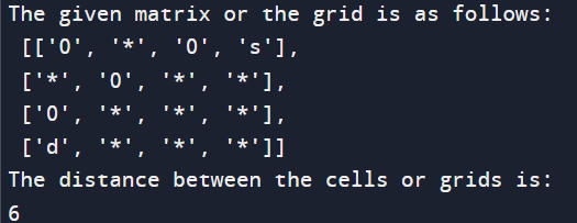
Still, the destination is only attainable if the line becomes empty and the destination cell is reached. Return an applicable index (e.g., -1).

The breadth-first hunt algorithm ensures that the shortest path is set up because it explores the grid in layers, meaning that shorter paths are considered ahead of longer ones.

Implementation

# The code for Python for implementing the code for finding the shortest distance between two cells in a matrix or grid.
# QUEItem is used for finding the current location and distance from the source location
class QUEItem:
def __init__(self, row, col, dist):
self.row = row
self.col = col
self.dist = dist
def __repr__(self):
return f"QItem({self.row}, {self.col}, {self.dist})"
def minimumdist(grid):
source = QUEItem(0, 0, 0)
# Finding the source to start from
for row in range(len(grid)):
for col in range(len(grid[row])):
if grid[row][col] == 's':
source.row = row
source.col = col
break
# For maintaining the location status.
visit = [[False for _ in range(len(grid[0]))]
for _ in range(len(grid))]
# applying BFS on matrix cells starting from a source
queue = []
queue.append(source)
visit[source.row][source.col] = True
while len(queue) != 0:
source = queue.pop(0)
# When the distance is found,
if (grid[source.row][source.col] == 'd'):
return source.dist
# The code for moving up.
if isValid(source.row - 1, source.col, grid, visit):
queue.append(QUEItem(source.row - 1, source.col, source.dist + 1))
visit[source.row - 1][source.col] = True
# The code for moving down.
if isValid(source.row + 1, source.col, grid, visit):
queue.append(QUEItem(source.row + 1, source.col, source.dist + 1))
visit[source.row + 1][source.col] = True
# The code for moving left.
if isValid(source.row, source.col - 1, grid, visit):
queue.append(QUEItem(source.row, source.col - 1, source.dist + 1))
visit[source.row][source.col - 1] = True
# The code for moving right.
if isValid(source.row, source.col + 1, grid, visit):
queue.append(QItem(source.row, source.col + 1, source.dist + 1))
visit[source.row][source.col + 1] = True
return -1
# The code for checking whether our move is valid or not.
def isValid(x, y, grid, visit):
if ((x >= 0 and y >= 0) and
(x < len(grid) and y < len(grid[0])) and
(grid[x][y] != '0') and (visit[x][y] == False)):
return True
return False
# The main code goes as follows:/
if __name__ == '__main__':
grid = [['0', '*', '0', 's'],
['*', '0', '*', '*'],
['0', '*', '*', '*'],
['d', '*', '*', '*']]
print("The given matrix or the grid is as follows:\n",grid)
print("The distance between the cells or grids is:")
print(minimum disk(grid))

Output:

The output of the above code is as follows:

Shortest distance between two cells in a matrix or grid

Explanation:

The purpose of this Python law is to find the shortest distance between two cells (' s' for source and 'd' for destination) in a given matrix or grid. The algorithm uses Breadth-First Search (BFS) to search the matrix totally and uses the QUEItem class to represent the current position and distance to the source.

Class QUEItem.

The QUEItem class is defined to store information about a matrix cell. It contains the attributes row, gap, and dist, which represent the row and column indicators and the distance to the source independently. The repr system is used for stoner-friendly descriptions of class cases.

Function minimumdist.

1. Source:

The process starts by initializing the source cell grounded on the letter 's' in the matrix.

2. Launch and BFS:

Produce a 2D array to control the incoming cells.

The row starts with the source cell.

The BFS process starts if the row isn't empty; the cells are removed from the line, and their neighbors are searched.

3. Cell discovery:

The function requires four possible movements: over, down, left, and right.

If a move is active (within a matrix boundary, mustn't be blocked by' 0', and doesn't reach it), a new QUEItem representing the neighbor is queued.

4. Appearance position:

Returns the path from the source to the destination if the destination cell ('d') is set up in the hunt.

5. The confirmation function is valid:

The isValid function checks whether a pass to a given cell is valid. This ensures that the indicators are within the matrix boundaries, the cell isn't confined to' 0', and the cell isn't dropped.

6. Special Section:

The main section defines the slice grid and minimizes.

Discussion

The algorithm searches the matrix totally by BFS, starting from the source cell. It uses a row to keep track of the hunt order and a navigation array to mark incoming cells. The BFS operation continues until the destination cell is reached and the distance is calculated. The isValid function ensures that only valid business is considered in the hunt.

Sample network

The illustration grid-handled a 4x4 matrix with' s' representing source cells, 'd' representing destination cells,' *' representing free cells,' 0' representing free cells, and' 0' representing free cells, ' representing free cells' representing free cells. The algorithm will find and publish the shortest distance between the source and destination cells.

This law illustrates the effective use of BFS to find the shortest path in a matrix, including the capability to rotate around constraints and find the optimal path between two specified cells.

Method 2:

The implementation of the above program using a deque library from collections package in python

from collections import deque
def sadist(mat, begin, endpoint):
    row, col = len(mat), len(mat[0])
    vis = [[False for _ in range(col)] for _ in range(row)]
    queue = deque([(begin, 0)])  # Each element in the queue is a tuple: (cell, distance)
    While queue:
        currcell, dist = queue.popleft()
        r, c = currcell
        # Checking whether the distance is reached.
        if currcell == endpoint:
            return dist
        # Explore neighbors (up, down, left, right)
        for dr, dc in [(-1, 0), (1, 0), (0, -1), (0, 1)]:
            new_row, new_col = r + dr, c + dc
            # Check if the neighbor is within the grid boundaries and not visited
            if 0 <= new_row < rows and 0 <= new_col < cols and not vis[new_row][new_col]:
                vis[new_row][new_col] = True
                queue.append(((new_row, new_col), dist + 1))
   # When the distance or the endpoint is not reachable, we return -1.
    return  -1

Output:

Explanation

The above Python law defines a point called sdist that calculates the shortest distance between two points in a given matrix using a breadth-first-search ( BFS) system. The characteristic takes three parameters: mat (a 2D matrix representing the grid), begin( a tuple representing the launch line), and endpoint( a tuple representing the target destination point).

The characteristic initializes variables to store the number of rows and columns within the matrix( row and gap), a 2D boolean array to tune visited cells( vies), and a deque( line) containing the place to begin and its distance, originally set to zero.

The middle of the set of rules is a BFS circle that iteratively explores cells in the matrix. Each new release dequeues a cell (currcell) and its distance (dist). Still, the characteristic without detention returns the space traveled, indicating that the shortest path has been determined if the present-day mobile is the destination point.

The point also explores bordering cells inside the up, down, left, and proper directions. It assesses whether each capacity circulates inside the matrix boundaries and has no longer been visited before. However, the mobile is marked as visited, and its equals, together with the streamlined distance, are enqueued for further inquiry if those situations are met.

Still, the characteristic returns 1, indicating that there may be no valid direction among the starting and finishing factors if the circle completes without locating the holiday spot point.

In precise, the sdist characteristic employs BFS to discover the shortest direction in expressions of the number of ways among a place to begin and a holiday spot factor in a given matrix. It makes use of a line to control the order of disquisition and a visited matrix to avoid reconsidering cells. The point returns the shortest distance if a valid path is observed and -1 in any other case.

Complexities:

Time complexity:

The time complexity of the BFS algorithm is generally expressed in terms of the number of knot edges in a graph or, in this case, an image. Let us denote the number of rows as R and the number of columns as C. In the worst case, the BFS algorithm is suitable to identify all the cells of the matrix. For each cell, the function finds its neighbors so that each cell has a constant process.

Therefore, the total time complexity of the sdist function is O(R * C), where R is the number of rows and C is the number of columns of the matrix.

Space complexity:

The data structure in which the information is stored in the BFS business is affected by the spatial complexity. In perpetration, the Boolean matrix vis is used to label the incoming cells, and the deque (line) is used to control the order of the hunt.

1. Visited matrix (vis)

The boolean matrix V confines R x C, representing the entire matrix. Therefore, the complex space for the input matrix is O (R * C).

2. Row (row)

In the worst case, the line can contain all the cells of the matrix. Thus, the space complexity for the line is also O(R * C).

The main difference between these two features is the space needed for the Boolean matrix; thus, the total space complexity of the function sdist is O(R * C).

In summary, the temporal complexity is O(R * C) and the spatial complexity is O(R * C), where R is the number of rows and C is the number of rows in the matrix.

Conclusion:

In conclusion, the problem of determining the shortest distance between two cells in a matrix or grid is an abecedarian algorithmic challenge with a wide range of practical operations. The main thing is to find the most effective route from a source cell into the specified destination cell, considering possible obstacles or blocked cells.

The Breadth-First Hunt (BFS) algorithm stands out as a popular and effective solution to this problem. It starts totally from the source cell and moves outward as a pass, searching for a shape. By using a line to control cell quests and a visited system to search for reused cells, BFS ensures that the shortest route is set up.

The introductory steps to troubleshoot this problem include initializing data structures, queuing source cells, performing BFS quests, checking destination cells, and calculating distances. These steps are frequently accompanied by an acknowledgment way to check that movement complies with matrix constraints and any specified constraints.

As similar, this problem finds operations in robotics, navigation systems, computer games, and control ways. Duly specifying the shortest distance between two points in the matrix is necessary to optimize the styles and form spatial opinions.

The two-handed Python law illustration serves to demonstrate the operation of the BFS algorithm to break the short-range problem. This illustration emphasizes the significance of systematic analysis, applicable data conformation, and careful confirmation for delicacy and effectiveness.

Next TopicSort an Array in Wave Form

← prev next →