COUNT OF ZEROES

Introduction

In laptop science and mathematics, matrices are regularly used to represent data in a structured way. Consider a matrix that is sorted in both row-wise and column-wise order.

In this manner, each row and each column of the matrix are looked after in ascending order. You are given such a matrix, and your undertaking is to determine the wide variety of zeros present in it. This hassle is more complex than counting zeroes in an ordinary matrix because the taken care of order lets in for a greener method.

Challenge:

The venture lies in exploiting the taken-care-of nature of the matrix to lay out an algorithm that optimally counts the zeroes without analyzing every detail personally. A brute-pressure method would include traversing the complete matrix and counting zeroes; however, this would not leverage the sorted order.

Optimized Approach:

To solve this problem effectively, you may use a binary seek-like technique to navigate through the matrix strategically. By starting from one nook of the matrix and making selections based on the houses of the looked-after matrix, it's far easier to decide the count of zeros in a more optimized manner.

Algorithm Steps:

1. Choose a start line, either the top-proper or the backside-left corner of the matrix.
2. Move in the direction of the alternative corner (both down and left or up and proper) based on the comparison of the contemporary detail with zero.
3. Utilize the sorted nature of the matrix to cast off entire rows or columns in each step.
4. Repeat this system until the complete matrix is blanketed.

Implementation:

Output:

The output of the above program is as follows: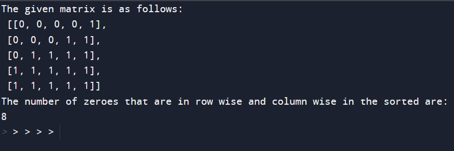

Explanation:

The supplied Python code aims to remember the wide variety of zeros in each sorted matrix that is ordered in both row-sensible and column-smart. Let's break down the code into its key additives and explain its capability: The feature `CZ (matrix)` takes a 2D matrix as input and returns the number of zeros in the matrix. The set of rules begins from the bottom-left nook of the matrix, and it iterates through the matrix in a way that leverages its sorted properties. Here's a step-by-step explanation of the code:

1. Initialization:

The variable `num` is set to five, representing the dimensions of the square matrix. - The variables `r` and `c` are initialized to `num - 1` and `0`, respectively, representing the starting point at the bottom-left corner of the matrix. - The variable `count number` is initialized to zero with a view to storing the total number of zeroes.

2. Main Loop:

The outer loop (`while c < num`) iterates over columns from left to right. - The internal loop (`while matrix[r][c] `) moves upwards inside the modern column until it reveals the first zero or reaches the top of the matrix (`r < zero`). - The matter of zeros inside the cutting-edge column is up to date by including ` (r 1) ` in the depend. This represents the number of zeros from the contemporary row to the lowest of the matrix within the given column.

3. Move to the Next Column:

After finishing a column, the outer loop increments `c`, transferring to the following column.

4. Result:

The characteristic returns the entire number of zeros within the matrix.

5. Example Matrix:

The supplied matrix is a 5x5 sorted matrix with varying numbers of zeros in each row and column.

In precis, the code efficiently counts the number of zeroes in a sorted matrix by using its residences. It employs a strategy that involves beginning from the bottom-left corner and shifting through the matrix in a manner that takes advantage of its taken care of nature, in the long run providing the whole depend on zeroes.

The provided Python program for calculating the number of zeros in a row-wise and column-wise ordered matrix shows an efficient method that takes advantage of the ordered properties of the matrix.

Challenging Times or Time Complexity:

Nested loops determine the complexity of a function through the core of the matrix. The outer wires return to the column, while the inner wires form a row again. In the worst case, the algorithm may traverse the entire matrix, resulting in a time complexity of O (m + n), where 'm' is the number of rows and 'n' is the number of rows. However, it is important to note that the inner loop already terminates when it encounters the first zero of the stacks. This property makes real-time complexity better than O (m + n) in many cases, especially when there are few zeros in the matrix.

Challenging Space or Space Complexity:

The spatial complexity of the program is very small and constant, O(1). The program uses a constant amount of extra space, regardless of the size of the input matrix. Variables used only for the calculation, such as `num,` `r,` `c,` and `count,` do not scale with the size of the input. In summary, the program is designed to be efficient in terms of time and space. The time complexity affects the shape of the theory, and the spatial complexity is very small and constant. This makes the algorithm suitable for large, ordered matrices without a significant increase in search requirements.

Conclusion:

In conclusion, the problem of zero counting in a row-wise and column-wise ordered matrix is solved by an estimated and efficient algorithm. The given Python program exploits the structure-property of the matrix to optimize the audit process.

Starting from the bottom left and moving through the matrix in the appropriate order, the algorithm correctly counts the number of zeros without examining each element individually. The time complexity of the program is O (m + n), where 'm' is the number of characters and 'n' is the number of characters.

Actual performance may also be better in cases of simple zero events due to the early termination of the inner loop when the first zero of the columns is encountered. Besides, the space complexity is constant, O (1). because the algorithm uses only fixed numbers of variables other than scale and input size.

This approach illustrates the importance of efficiently solving problems with algorithmic design, especially when dealing with structured data such as structured matrices. The ability to manipulate the unique characteristics of the data allows for more customized solutions, making algorithms suitable for handling large matrices with improved resource efficiency.

Overall, the presented algorithm is a practical and efficient solution to the problem of zero counting in a structured matrix and contributes to the understanding of the algorithmic approaches for matrix transformation and analysis.