AVL Trees Operations

In 1962, GM Adelson-Velsky and EM Landis created the AVL Tree. To honors the people who created it, the tree is known as AVL.

The definition of an AVL tree is a height-balanced binary search tree in which each node has a balance factor that is determined by deducting the height of the node's right sub tree from the height of its left sub tree.

If each node's balance factor falls between -1 and 1, the tree is considered to be balanced; otherwise, the tree needs to be balanced.

Balance Factor

Balance Factor (k) = height (left(k)) - height (right(k))

The left sub-tree is one level higher than the right sub-tree if the balancing factor of any node is 1.
Any node with a balance factor of zero indicates that the heights of the left and right sub trees are equal.
If a node's balancing factor is negative one, the left sub-tree is one level behind the right sub-tree.
In the following figure, an AVL tree is presented. We can observe that each node's associated balancing factor ranges from -1 to +1. So, it is an illustration of an AVL tree.

Why use AVL Trees?

The majority of BST operations, including search, max, min, insert, delete, and others, require O(h) time, where h is the BST's height. For a skewed Binary tree, the cost of these operations can increase to O(n). We can provide an upper bound of O(log(n)) for all of these operations if we make sure that the height of the tree stays O(log(n)) after each insertion and deletion. An AVL tree's height is always O(log(n)), where n is the tree's node count.

Operations on AVL Trees

Due to the fact that, AVL tree is also a binary search tree hence, all the operations are conducted in the same way as they are performed in a binary search tree. Searching and traversing do not lead to the violation in property of AVL tree. However, the actions that potentially break this condition are insertion and deletion; as a result, they need to be reviewed.

Insertion
Deletion

Insertion in AVL Trees

We must add some rebalancing to the typical BST insert procedure to ensure that the provided tree stays AVL after each insertion.

The following two simple operations (keys(left) key(root) keys(right)) can be used to balance a BST without going against the BST property.

Rotate left
Rotate right

The tree's T1, T2, and T3 subtrees are rooted with either y (on the left side) or x. (on the right side)
     y                                          x
    / \     Right Rotation          /  \
   x   T3   - - - - - - - >             T1    y 
  / \       < - - - - - - -                  / \
 T1  T2     Left Rotation        T2  T3
The order of the keys in the two trees mentioned above is as follows:
keys(T1) < key(x) < keys(T2) < key(y) < keys(T3)
Therefore, no BST property has been broken.

The steps to take for insertion are:

Let w be the newly added node.
carry out a typical BST insert for w.
Find the first imbalanced node by moving up starting at w. Assume that z is the initial imbalanced node, y is z's kid who arrives on the path from w to z, and x is z's grandchild that arrives on the aforementioned path.
Rotate the z-rooted subtree in the proper directions to rebalance the tree. As x, y, and z can be ordered in 4 different ways, there may be 4 potential scenarios that need to be addressed.
The four potential configurations are as follows:
- Left Left Case: y is z's left child and x's left child.
- Left Right Case: z's right child and x's right child.
- Right Right Case: y is z's right child and x's left child.
- Right Right Case: y is z's right child and x's left child.

The procedures to be carried out in the four circumstances indicated above are listed below. In every instance, we only need to rebalance the subtree rooted with z, and the entire tree will be balanced as soon as the height of the subtree rooted with z equals its pre-insertion value (with the proper rotations).

1. Left Left Case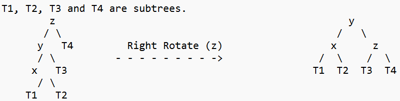

2. Left Right Case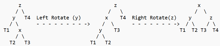

3. Right Right Case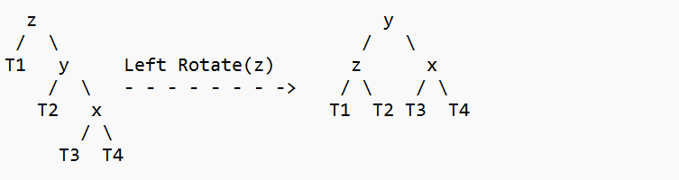

4. Right Left Case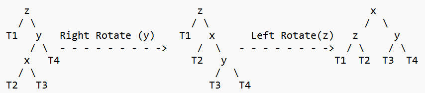

Approach for Insertion

The concept is to utilize recursive BST insert, where after insertion, we receive bottom-up pointers to each ancestor individually. Therefore, to go up, we don't require a parent pointer. The recursive code itself ascends and visits every node that was previously inserted.

To put the concept into practise, adhere to the procedures listed below:

Carry out the standard BST insertion.
The newly inserted node's ancestor must be the current node. The current node's height should be updated.
Find the current node's balancing factor (left subtree height minus right subtree height).
The current node is imbalanced and we are either in the Left Left case or Left Right case if the balance factor is larger than 1. Compare the newly inserted key with the key at the left subtree root to determine if it is left left case or not.

Program for insertion:

// C program to insert a node in AVL tree
#include<stdio.h>
#include<stdlib.h>

// An AVL tree node
struct Node
{
	int key;
	struct Node *left;
	struct Node *right;
	int height;
};

// A utility function to get the height of the tree
int height(struct Node *N)
{
	if (N == NULL)
		return 0;
	return N->height;
}

// A utility function to get maximum of two integers
int max(int a, int b)
{
	return (a > b)? a : b;
}

/* Helper function that allocates a new node with the given key and
	NULL left and right pointers. */
struct Node* newNode(int key)
{
	struct Node* node = (struct Node*)
						malloc(sizeof(struct Node));
	node->key = key;
	node->left = NULL;
	node->right = NULL;
	node->height = 1; // new node is initially added at leaf
	return(node);
}

/ / A utility function to right rotate subtree rooted with y
// See the diagram given above.
struct Node *rightRotate(struct Node *y)
{
	struct Node *x = y->left;
	struct Node *T2 = x->right;

	// Perform rotation
	x->right = y;
	y->left = T2;

	// Update heights
	y->height = max(height(y->left),
					height(y->right)) + 1;
	x->height = max(height(x->left),
					height(x->right)) + 1;

	// Return new root
	return x;
}

// A utility function to left rotate subtree rooted with x
// See the diagram given above.
struct Node *leftRotate(struct Node *x)
{
	struct Node *y = x->right;
	struct Node *T2 = y->left;

	// Perform rotation
	y->left = x;
	x->right = T2;

	// Update heights
	x->height = max(height(x->left),
					height(x->right)) + 1;
	y->height = max(height(y->left),
					height(y->right)) + 1;

	// Return new root
	return y;
}

// Get Balance factor of node N
int getBalance(struct Node *N)
{
	if (N == NULL)
		return 0;
	return height(N->left) - height(N->right);
}

// Recursive function to insert a key in the subtree rooted
// with node and returns the new root of the subtree.
struct Node* insert(struct Node* node, int key)
{
	/* 1. Perform the normal BST insertion */
	if (node == NULL)
		return(newNode(key));

	if (key < node->key)
		node->left = insert(node->left, key);
	else if (key > node->key)
		node->right = insert(node->right, key);
	else // Equal keys are not allowed in BST
		return node;

	/* 2. Update height of this ancestor node */
	node->height = 1 + max(height(node->left),
						height(node->right));

	/* 3. Get the balance factor of this ancestor
		node to check whether this node became
		unbalanced */
	int balance = getBalance(node);

	// If this node becomes unbalanced, then
	// there are 4 cases

	// Left Left Case
	if (balance > 1 && key < node->left->key)
		return rightRotate(node);

	// Right Right Case
	if (balance < -1 && key > node->right->key)
		return leftRotate(node);

	// Left Right Case
	if (balance > 1 && key > node->left->key)
	{
		node->left = leftRotate(node->left);
		return rightRotate(node);
	}

	// Right Left Case
	if (balance < -1 && key < node->right->key)
	{
		node->right = rightRotate(node->right);
		return leftRotate(node);
	}

	/* return the (unchanged) node pointer */
	return node;
}

// A utility function to print preorder traversal
// of the tree.
// The function also prints height of every node
void preOrder(struct Node *root)
{
	if(root != NULL)
	{
		printf("%d ", root->key);
		preOrder(root->left);
		preOrder(root->right);
	}
}

/* Driver program to test above function*/
int main()
{
struct Node *root = NULL;

/* Constructing tree given in the above figure */
root = insert(root, 10);
root = insert(root, 20);
root = insert(root, 30);
root = insert(root, 40);
root = insert(root, 50);
root = insert(root, 25);

/* The constructed AVL Tree would be
	            30
		/ \
	          20 40
	     / \	 \
	    10 25   50
*/

printf("Preorder traversal of the constructed AVL"
		" tree is \n");
preOrder(root);
return 0;
}

Output

Preorder traversal of the constructed AVL tree is 
30 20 10 25 40 50
......................................................................................
Process executed in 1.22 seconds
Press any key to continue

Explanation

Only a few points are updated during the rotation operations (left and right rotate), hence the time required is constant. It also takes a consistent amount of time to update the height and obtain the balancing factor. As a result, the AVL insert has the same temporal complexity as the BST insert, which is O(h), where h is the tree's height. The height is O since the AVL tree is balanced (Logn). Thus, the AVL insert's temporal complexity is O(Logn).

Comparing it with Red Black Tree

Red Black Tree:

The additional bit that each node possesses in a red-black tree, a type of self-balancing binary search tree, is frequently understood as the color (red or black). The balance of the tree is maintained throughout insertions and deletions thanks to the employment of these colors. Although the tree's balance is not ideal, it is sufficient to cut down on searching time and keep it at or below O(log n), where n is the total number of tree components. The Rudolf Bayer invented this tree in 1972.

All fundamental operations may be completed in O(log n) time by using the AVL tree and other self-balancing search trees like Red Black. Compared to Red-Black Trees, AVL Trees are more evenly distributed, although they may result in more rotations during insertion and deletion. Red Black trees are thus recommended if your application includes frequent, frequent insertions and removals. Additionally, the AVL tree should be chosen over the Red Black Tree if searches are performed more often and insertions and deletions are less frequent.

Deletion in AVL Trees

We must add some rebalancing to the typical BST delete procedure to ensure that the supplied tree stays AVL after each deletion. The following two simple operations (keys(left) key(root) keys(right)) can be used to rebalance a BST without going against the BST property.

Left Rotation
Right Rotation

The tree's T1, T2, and T3 subtrees are rooted with y (on the left side) or x. (on right side)

The order of the keys in the two trees mentioned above is as follows:

keys(T1) < key(x) < keys(T2) < key(y) < keys(T3)

Let w represent the removed node:

Carry out the typical BST delete for w.
Find the first imbalanced node by moving up starting at w. Let y be the bigger height child of z, x be the larger height child of y, and z be the initial imbalanced node. The definitions of x and y change from insertion here, as you will see.
Rotate the z-rooted sub tree in the proper directions to rebalance the tree. As x, y, and z can be ordered in 4 different ways, there may be 4 potential scenarios that need to be addressed. The four potential configurations are as follows:
- Left Left Case: y is the left child of z and x is the left child of y
- y is the left child of z and x is the right child of y. (Left Right Case)
- y is z's right-hand kid, and X is y's right-hand child (Right Right Case)
- Z's right kid is y, whereas x is y's left child (Right Left Case)

The procedures to be carried out in the aforementioned 4 circumstances are as follows, just like insertion. Be aware that, unlike insertion, repairing node z won't result in a full fix of the AVL tree.

1. Left Left Case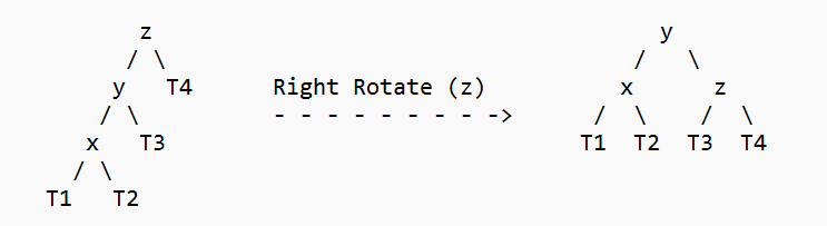

2. Left Right Case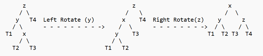

3. Right Right Case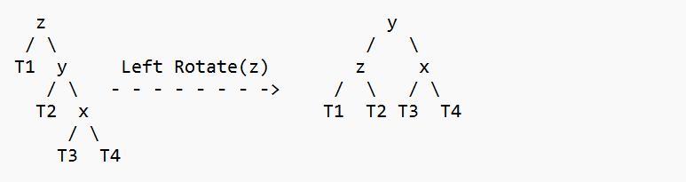

4. Right Left Case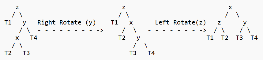

In contrast to insertion, rotation at z may be followed by rotation at z's ancestors in deletion. In order to get to the root, we must thus keep following the path.

Approach for Deletion

The AVL Tree Deletion C implementation is provided below. The recursive BST delete is the foundation of the following C implementation. After the deletion in the recursive BST delete, we receive bottom-up pointers to each ancestor in turn. Therefore, ascending doesn't require the parent pointer. The recursive code itself ascends and accesses each of the removed node's ancestors.

Carry out the standard BST delete.
One of the ancestors of the removed node must be the current node. The current node's height should be updated.
Find the current node's balancing factor (left sub tree height minus right sub tree height).
The current node is imbalanced and we are either in Left Left case or Left Right case if the balance factor is larger than 1. Obtain the left sub tree's balancing factor to determine if the situation is Left Left or Left Right. If the left sub tree's balance factor is larger than or equal to 0, it is left left case; otherwise, it is left right case.
The present node is imbalanced if the balancing factor is less than -1, and we are either in Right Left case or Right Right case. Obtain the balancing factor for the right sub tree to determine if it is the Right Right case or the Right Left case. Right Right case is indicated if the balancing factor of the right sub tree is less than or equal to 0, else Right Left case.

Program for deletion in C

// C program to delete a node from AVL Tree
#include<stdio.h>
#include<stdlib.h>
// An AVL tree node
struct Node
{
	int key;
	struct Node *left;
	struct Node *right;
	int height;
};

// A utility function to get maximum of two integers
int max(int a, int b);

// A utility function to get height of the tree
int height(struct Node *N)
{
	if (N == NULL)
		return 0;
	return N->height;
}

// A utility function to get maximum of two integers
int max(int a, int b)
{
	return (a > b)? a : b;
}

/* Helper function that allocates a new node with the given key and
	NULL left and right pointers. */
struct Node* newNode(int key)
{
	struct Node* node = (struct Node*)
						malloc(sizeof(struct Node));
	node->key = key;
	node->left = NULL;
	node->right = NULL;
	node->height = 1; // new node is initially added at leaf
	return(node);
}

// A utility function to right rotate subtree rooted with y
// See the diagram given above.
struct Node *rightRotate(struct Node *y)
{
	struct Node *x = y->left;
	struct Node *T2 = x->right;

	// Perform rotation
	x->right = y;
	y->left = T2;

	// Update heights
	y->height = max(height(y->left), height(y->right))+1;
	x->height = max(height(x->left), height(x->right))+1;

	// Return new root
	return x;
}

// A utility function to left rotate subtree rooted with x
// See the diagram given above.
struct Node *leftRotate(struct Node *x)
{
	struct Node *y = x->right;
	struct Node *T2 = y->left;

	// Perform rotation
	y->left = x;
	x->right = T2;

	// Update heights
	x->height = max(height(x->left), height(x->right))+1;
	y->height = max(height(y->left), height(y->right))+1;

	// Return new root
	return y;
}

// Get Balance factor of node N
int getBalance(struct Node *N)
{
	if (N == NULL)
		return 0;
	return height(N->left) - height(N->right);
}

struct Node* insert(struct Node* node, int key)
{
	/* 1. Perform the normal BST rotation */
	if (node == NULL)
		return(newNode(key));

	if (key < node->key)
		node->left = insert(node->left, key);
	else if (key > node->key)
		node->right = insert(node->right, key);
	else // Equal keys not allowed
		return node;

	/* 2. Update height of this ancestor node */
	node->height = 1 + max(height(node->left),
						height(node->right));

	/* 3. Get the balance factor of this ancestor
		node to check whether this node became
		unbalanced */
	int balance = getBalance(node);

	// If this node becomes unbalanced, then there are 4 cases

	// Left Left Case
	if (balance > 1 && key < node->left->key)
		return rightRotate(node);

	// Right Right Case
	if (balance < -1 && key > node->right->key)
		return leftRotate(node);

	// Left Right Case
	if (balance > 1 && key > node->left->key)
	{
		node->left = leftRotate(node->left);
		return rightRotate(node);
	}

	// Right Left Case
	if (balance < -1 && key < node->right->key)
	{
		node->right = rightRotate(node->right);
		return leftRotate(node);
	}

	/* return the (unchanged) node pointer */
	return node;
}

/* Given a non-empty binary search tree, return the
node with minimum key value found in that tree.
Note that the entire tree does not need to be
searched. */
struct Node * minValueNode(struct Node* node)
{
	struct Node* current = node;

	/* loop down to find the leftmost leaf */
	while (current->left != NULL)
		current = current->left;

	return current;
}

// Recursive function to delete a node with given key
// from subtree with given root. It returns root of
// the modified subtree.
struct Node* deleteNode(struct Node* root, int key)
{
	// STEP 1: PERFORM STANDARD BST DELETE

	if (root == NULL)
		return root;

	// If the key to be deleted is smaller than the
	// root's key, then it lies in left subtree
	if ( key < root->key )
		root->left = deleteNode(root->left, key);

	// If the key to be deleted is greater than the
	// root's key, then it lies in right subtree
	else if( key > root->key )
		root->right = deleteNode(root->right, key);

	// if key is same as root's key, then This is
	// the node to be deleted
	else
	{
		// node with only one child or no child
		if( (root->left == NULL) || (root->right == NULL) )
		{
			struct Node *temp = root->left ? root->left :
											root->right;

			// No child case
			if (temp == NULL)
			{
				temp = root;
				root = NULL;
			}
			else // One child case
			*root = *temp; // Copy the contents of
							// the non-empty child
			free(temp);
		}
		else
		{
			// node with two children: Get the inorder
			// successor (smallest in the right subtree)
			struct Node* temp = minValueNode(root->right);

			// Copy the inorder successor's data to this node
			root->key = temp->key;

			// Delete the inorder successor
			root->right = deleteNode(root->right, temp->key);
		}
	}

	// If the tree had only one node then return
	if (root == NULL)
	return root;

	// STEP 2: UPDATE HEIGHT OF THE CURRENT NODE
	root->height = 1 + max(height(root->left),
						height(root->right));

	// STEP 3: GET THE BALANCE FACTOR OF THIS NODE (to
	// check whether this node became unbalanced)
	int balance = getBalance(root);

	// If this node becomes unbalanced, then there are 4 cases

	// Left Left Case
	if (balance > 1 && getBalance(root->left) >= 0)
		return rightRotate(root);

	// Left Right Case
	if (balance > 1 && getBalance(root->left) < 0)
	{
		root->left = leftRotate(root->left);
		return rightRotate(root);
	}

	// Right Right Case
	if (balance < -1 && getBalance(root->right) <= 0)
		return leftRotate(root);

	// Right Left Case
	if (balance < -1 && getBalance(root->right) > 0)
	{
		root->right = rightRotate(root->right);
		return leftRotate(root);
	}

	return root;
}

// A utility function to print preorder traversal of
// the tree.
// The function also prints height of every node
void preOrder(struct Node *root)
{
	if(root != NULL)
	{
		printf("%d ", root->key);
		preOrder(root->left);
		preOrder(root->right);
	}
}

/* Driver program to test above function*/
int main()
{
struct Node *root = NULL;

/* Constructing tree given in the above figure */
	root = insert(root, 9);
	root = insert(root, 5);
	root = insert(root, 10);
	root = insert(root, 0);
	root = insert(root, 6);
	root = insert(root, 11);
	root = insert(root, -1);
	root = insert(root, 1);
	root = insert(root, 2);

	/* The constructed AVL Tree would be
			9
		/ \
		1 10
		/ \	 \
	0 5	 11
	/ / \
	-1 2 6
	*/

	printf("Preorder traversal of the constructed AVL "
		"tree is \n");
	preOrder(root);

	root = deleteNode(root, 10);

	/* The AVL Tree after deletion of 10
			1
		/ \
		0 9
		/	 / \
	-1 5	 11
		/ \
		2 6
	*/

	printf("\nPreorder traversal after deletion of 10 \n");
	preOrder(root);

	return 0;
}

Output

Preorder traversal of the constructed AVL tree is 
9 1 0 -1 5 2 6 10 11 
Preorder traversal after deletion of 10 
1 0 -1 9 5 2 6 11
.....................................................................................
Process executed in 2.11 seconds
Press any key to continue

Explanation

The time required is constant since only a small number of points are updated during the rotation operations (left and right rotate). Getting the balance factor and updating the height both take time. As a result, the AVL delete has O(h), where h is the height of the tree, the same temporal complexity as the BST delete. The height is O as a result of the AVL tree's balance (Logn). Thus, the temporal complexity of AVL delete is O. (Log n).

The benefits of AVL trees:

The balance of height is constant.
N is the number of nodes, and height never exceeds logN.
Compared to a binary search tree, it provides a superior search.
It has the ability to balance itself.

Summary

These binary search trees are self-balancing.
Balancing Factor values fall between -1 and +1.
When the balancing factor exceeds the range, rotations must be made.
Time for insert, delete, and search is O. (log N).
Avl trees are typically employed in situations where searches occur more frequently than inserts and deletions.

Next TopicLimitations of Stack in Data Structures

← prev next →