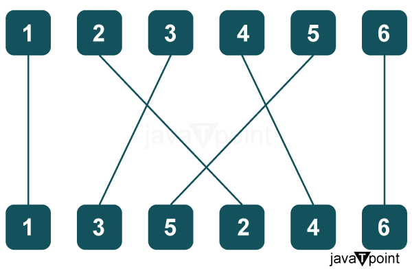
Counting Inversions Problem in Data Structure

A primary data structure used in programming and computer science is an array. Analyzing an array's "sorted" or "unsorted" status is frequently helpful. Counting the number of inversions in the array is one way to measure this. When two items in an array are out of order with respect to one another, this is known as an inversion. Analyzing the number of inversions provides information about how unsorted an array is. This article will examine various methods that may be used to count the inversions in an array effectively. These algorithms include an O(N^2) nested loop method that is straightforward and an O(N log N) divide-and-conquer merge sort-based strategy that is more effective. Counting inversions has applications in fields like data analysis to quantify disordered datasets. We will discuss how to implement inversion counting and its critical applications.

Approach 1: Brute Force

When I first learned about counting inversions in arrays, a simple "brute force" solution with nested loops made intuitive sense. An inversion is when a pair of elements are out of order relative to each other, like having 3 appear before 1 in an array. To count all inversions, we could compare each element to all the ones to its right.

The code below shows how this might work. There are two for loops - the outer loop i goes from the start to the end of the array, and the inside loop j goes from i+1 to the end. Inside the inner loop, it compares arr[i] and arr[j], incrementing the count if arr[i] is bigger than arr[j] since that's an inversion.

By the end, the count variable tallies up all inversion pairs. This nested loop brute force solves the problem and is easy to understand. But it could be more efficient, needing to check every single pair taking O(N^2) time. As the array gets more significant, this quickly balloons in computation.

Still, starting with the brute-force solution is helpful. It provides a simple baseline before diving into fancier algorithms. Walking through the naive approach can build intuition before tackling divide-and-conquer solutions with better O(N log N) speed. Beginning in familiar territory lets you ease into core concepts, even if, in practice, you'd avoid the brute force tactics.

Output:

Number of inversions: 6

Explanation:

• The function count_inversions_bruteforce takes an array arr as input
• It initializes a variable count to 0 to store the number of inversions
• It calculates the length of the array using n = len(arr)
• It runs two nested for loops:
• The outer loop goes from 0 to n-1, with i as the index
• The inner loop goes from i+1 to n, with j as the index
• Inside the inner loop, it compares arr[i] and arr[j]
• If arr[i] > arr[j], it means an inversion is found. So, it increments the count by 1
• After the nested loops finish, the count contains the total inversions
• The function returns the count
• In the main block:
• An example array arr is defined
• count_inversions_bruteforce is called on arr
• The number of inversions is printed
• This implements the simple O(N^2) algorithm to count inversions using nested loops
• It compares each element with all elements to the right, incrementing count when an inversion is found
• Time complexity is O(N^2) as there are two nested loops iterating the array

A primary data structure used in programming and computer science is an array. Analyzing an array's "sorted" or "unsorted" status is frequently helpful. Counting the number of inversions in the array is one way to measure this. When two items in an array are out of order with respect to one another, this is known as an inversion. Analyzing the number of inversions provides information about how unsorted an array is. This article will examine various methods that may be used to count the inversions in an array effectively. These algorithms include an O(N^2) nested loop method that is straightforward and an O(N log N) divide-and-conquer merge sort-based strategy that is more effective. Counting inversions has applications in fields like data analysis to quantify disordered datasets. We will discuss how to implement inversion counting and its key applications.

Approach 2: Merge Sort Method

Counting inversions in an array can be sped up significantly using a divide and conquer approach like merge sort. The key insight is that when merging two sorted subarrays, we can efficiently count the number of inversions between elements of the two subarrays. This allows us to count inversions in overall O(N log N) time.

The code below implements an inversion counter using merge sort. It consists of a merge function that handles merging two sorted subarrays and counts inversions between them. This merge function is called from a recursive merge sort function that splits the array into halves, recursively sorts them, and then merges the two sorted halves while counting split inversions.

By dividing the problem and only counting inversions during the merge steps, the overall time complexity is reduced from O(N^2) in the brute force approach to O(N log N) with merge sort. This speedup allows inversion counting to scale to large arrays. While the code may appear complicated initially, walking through it will reveal how to divide and conquer fundamentally reduces the complexity. In this introduction, we will unpack how to merge sort with inversion counting works at a high level before going into its implementation details.

Output:

Number of inversions: 6

Explanation

• It implements inversion counting using merge sort
• merge function does the following:
• Takes array, temp array, left/right indices
• Maintains indices i, j, k
• Keeps merging left and right sorted subarrays
• If the element from left is <= element from right, copies to temp
• Else copies right element, increments inv_count by mid-i+1 (inversions with remaining left)
• Returns inv_count for merge step
• merge_sort_and_count function:
• Base case: If left >= right, return
• Recursively sort and count the left half
• Recursively sort and count the right half
• Merge sorted halves and count split inversions
• Return total inversions
• Main count_inversions_merge_sort function:
• Creates temp array
• Calls merge_sort_and_count on full array
• Returns total inversion count
• Main block:
• Runs on sample array
• Prints number of inversions
• Merge sort divides the array into subproblems and merges sorted halves
• Counting happens during the merge step
• Overall time complexity is O(N log N)

Conclusion

In summary, counting the number of inversions in an array provides a valuable metric of how disordered or unsorted an array is. We explored two approaches to count inversions - a simple O(N^2) nested looping brute force method and a more efficient O(N log N) divide and conquer merge sort algorithm.

The brute force approach using two nested for loops to compare all pairs is straightforward but infeasible for significant inputs due to its quadratic time complexity. By dividing the array and counting inversions only during the merging of sorted subarrays, merge sort reduces the complexity to linearithmic time.

Counting inversions has applications in fields like data analysis and machine learning to quantify disorder in datasets. It can identify issues like anomalies or deviations from an expected ordering. The algorithms discussed provide ways to implement inversion counts efficiently, even for extensive real-world data.

In the future, it would be interesting to study parallelized implementations of inversion counting that leverage multiple processors. The divide and conquer nature of merge sort lends itself well to parallelization. Applying similar techniques to inversion counting could further boost its speed and scalability.