Sorting Techniques in Data Structures

Introduction:

Sorting is a fundamental computer science operation that entails putting a group of objects in a specific order. It is extensively utilised in many different applications, including database management, data analysis, and searching. In data structures, different sorting techniques are employed to organize and manipulate large sets of data efficiently.

Sorting Techniques:

There are various sorting techniques, which are listed in the table below:

Algorithm	Description	Time Complexity	Space Complexity
Bubble Sort	Compares nearby elements, swaps any that are out of order, and repeats until the array is sorted.	O(n^2)	O(1)
Selection Sort	Divides the input array into two sections: one that is sorted and one that is not. It does this by repeatedly choosing the smallest element in the unsorted zone and moving it to the sorted region.	O(n^2)	O(1)
Insertion Sort	By continuously inserting each unsorted element into the appropriate location within the sorted subarray, the final sorted array is built one element at a time.	O(n^2)	O(1)
Merge Sort	Merge Sort splits the input array in half, sorts each half iteratively, and then combines the two sorted halves to create the final sorted array.	O(n log n)	O(n)
Quick Sort	Selects a pivot element and divides the array so that everything that is smaller than the pivot is put in front of it, and everything that is bigger than the pivot is put in back. The subarrays prior to and following the pivot are then sorted recursively.	O(n log n)	O(log n)
Heap Sort	Creates a max-heap from the input array, removes the highest element from the heap periodically, swaps it for the last element, and modifies the heap until the array is sorted.	O(n log n)	O(1)
Counting Sort	creates a count array to keep track of how many distinct elements there are in the input array. Then it determines the position of each element by calculating the cumulative sum of counts.	O(n + k)	O(n + k)
Bucket Sort	Divides the input array into a set of buckets, where each bucket represents a range of values. It distributes elements into the respective buckets based on their values. Then, each bucket is sorted separately, usually using a different sorting method.	O(n^2) or O(n + k)	O(n)
Radix Sort	Sorts elements by processing individual digits or characters of the elements from the least significant digit (LSD) to the most significant digit (MSD). As a subroutine, it may employ a reliable sorting algorithm.	O(d * (n + k))	O(n + k)

Bubble Sort:

The straightforward sorting method known as "Bubble Sort" analyses neighbouring elements, iteratively goes over the list, and swaps out any elements that are out of order. To sort the complete list, repeat this step.

Example:

Let's consider an array of integers: {5, 2, 8, 12, 3}.

In the first pass, the algorithm compares 5 and 2, swaps them, and then compares 5 and 8 (no swap). Next, it compares 8 and 12 (no swap), and finally, 12 and 3, resulting in a swap. The array becomes: {2, 5, 8, 3, 12}.
In the second pass, the algorithm compares 2 and 5 (no swap), 5 and 8 (no swap), and 8 and 3, leading to a swap. The array becomes: {2, 5, 3, 8, 12}.
In the third pass, the algorithm compares 2 and 5 (no swap), 5 and 3, resulting in a swap. The array becomes: {2, 3, 5, 8, 12}.
In the fourth pass, all elements are already sorted, so no swaps occur.

Program:

#include <iostream>
using namespace std;

void bubbleSort(int arr[], int size) {
    for (int i = 0; i < size - 1; ++i) {
        for (int j = 0; j < size - i - 1; ++j) {
            if (arr[j] > arr[j + 1]) {
                // Swap the elements
                int temp = arr[j];
                arr[j] = arr[j + 1];
                arr[j + 1] = temp;
            }
        }
    }
}

int main() {
    int arr[] = {5, 2, 8, 12, 3};
    int size = sizeof(arr) / sizeof(arr[0]);

    bubbleSort(arr, size);

    cout << "Sorted array: ";
    for (int i = 0; i < size; ++i) {
        cout << arr[i] << " ";
    }

    return 0;
}

Explanation:

The bubbleSort function takes an array (arr) and its size (size) as input. It iterates across the array and compares nearby elements using nested loops.

A swap is carried out if the current element is larger than the following element. Until the largest element "bubbles" to the end of the array, this process is repeated.

An array named arr is initialised with some values in the main function, and the size of the array is determined using the sizeof operator.

The bubbleSort function is then called, passing the array and its size.

Program Output:

Selection Sort:

Selection Sort is a sorting algorithm that uses in-place comparisons. It separates the input array into two sections, one that is sorted and the other that is not. The algorithm chooses the least (or maximum) element from the unsorted part of the portion and inserts it at the start of the sorted part of the portion in each iteration.

Example:

Consider the same array of integers: {5, 2, 8, 12, 3}.

In the first iteration, the algorithm finds the minimum element as 2 and swaps it with the first element. The array becomes: {2, 5, 8, 12, 3}.
In the second iteration, the algorithm finds the minimum element in the unsorted portion (starting from the second element) as 3 and swaps it with the second element. The array becomes: {2,5, 8, 12, 3}.
In the third iteration, the algorithm determines that the third element is the minimum element in the unsorted segment, beginning from that element, and swaps it with that element. The array becomes: {2, 3, 8, 12, 5}.
In the fourth iteration, the algorithm finds the minimum element in the unsorted portion (starting from the fourth element) as 5 and swaps it with the fourth element. The array becomes: {2, 3, 5, 12, 8}.
In the fifth iteration, there is only one element left in the unsorted portion, so no swaps occur.

Program:

#include <iostream>
using namespace std;

void selectionSort(int arr[], int size) {
    for (int i = 0; i < size - 1; ++i) {
        int minIndex = i;
        for (int j = i + 1; j < size; ++j) {
            if (arr[j] < arr[minIndex]) {
                minIndex = j;
            }
        }
        // Swap the minimum element with the current element
        int temp = arr[minIndex];
        arr[minIndex] = arr[i];
        arr[i] = temp;
    }
}

int main() {
    int arr[] = {5, 2, 8, 12, 3};
    int size = sizeof(arr) / sizeof(arr[0]);

    selectionSort(arr, size);

    cout << "Sorted array: ";
    for (int i = 0; i < size; ++i) {
        cout << arr[i] << " ";
    }

    return 0;
}

Explanation:

The selectionSort function takes an array (arr) and its size (size) as input. It uses nested loops to iterate through the array. The inner loop searches the remaining unsorted portion of the array for the minimum element while the outer loop chooses the current member.

When the inner loop is finished, the outer loop's current element is switched out for the minimum element. By doing this, it is ensured that the minimal element is shifted to the proper position in the sort.

The size of the array is determined by using the sizeof operator once an array named arr is initialised in the main function with some data. The selectionSort function is then called, passing the array and its size.

Program Output:

Insertion Sort:

Insertion Sort is a straightforward sorting algorithm that creates the finished sorted array one item at a time. One element at a time, iteratively taking into account the input array, it inserts each element into the sorted portion of the array in the proper place.

Example:

Let's use the same array of integers: {5, 2, 8, 12, 3}.

In the first iteration, the algorithm considers 5 as the first element, which is already sorted, so no changes occur.
In the second iteration, the algorithm considers 2 and inserts it before 5, resulting in {2, 5, 8, 12, 3}.
In the third iteration, the algorithm takes into account 8, which is already in the right place.
In the fourth iteration, the algorithm takes into account 12, which is already in the right position.
In the fifth iteration, the algorithm considers 3 and inserts it between 2 and 5, resulting in {2, 3, 5, 8, 12}.

Program:

#include <iostream>
using namespace std;


void insertionSort(int arr[], int size) {
    for (int i = 1; i < size; ++i) {
        int key = arr[i];
        int j = i - 1;

        while (j >= 0 && arr[j] > key) {
            arr[j + 1] = arr[j];
            j--;
        }

        arr[j + 1] = key;
    }
}

int main() {
    int arr[] = {5, 2, 8, 12, 3};
    int size = sizeof(arr) / sizeof(arr[0]);

    insertionSort(arr, size);

    cout << "Sorted array: ";
    for (int i = 0; i < size; ++i) {
        cout << arr[i] << " ";
    }

    return 0;
}

Explanation:

The insertionSort function takes an array arr and its size size as input. It begins comparing with the elements in the array's sorted portion with the second element (i = 1). It then iterates backward (j = i - 1) through the sorted part of the array, shifting the elements to the right if they are greater than the key value.

The inner while loop continues until either j becomes negative or the element at index j is not greater than key. This loop shifts the elements to the right to make space for the key value in its correct sorted position.

After the while loop, the key value is inserted into the sorted position (arr[j + 1] = key). The array's elements are processed one at a time until all of them have been.

The sizeof operator is used in the main function to determine the array's size after initialising an array called arr with certain values.The insertionSort function is then called, passing the array and its size.

Program Output:

Merge Sort:

Merge Sort is a divide-and-conquer algorithm that divides the input array into smaller subarrays, sorts them, and then combines them to produce a sorted output. It uses a "merge" operation to combine the smaller sorted subarrays into a larger sorted array.

Example:

Consider the array of integers: {5, 2, 8, 12, 3}.

The algorithm divides the array into two halves: {5, 2} and {8, 12, 3}.
It further divides the first half into {5} and {2}.
The individual elements are already sorted, so the algorithm merges {5} and {2} to obtain {2, 5}.
Similarly, the second half {8, 12, 3} is divided into {8} and {12, 3}, and then further into {12} and {3}.
The subarrays {8} and {12} are merged to obtain {8, 12}.
Finally, the subarrays {2, 5} and {8, 12, 3} are merged to obtain the sorted array {2, 3, 5, 8, 12}.

Program:

#include<iostream>
using namespace std;

void merge(int arr[], int left, int mid, int right) {
    int n1 = mid - left + 1;
    int n2 = right - mid;

    int L[n1], R[n2];

    for (int i = 0; i < n1; ++i)
        L[i] = arr[left + i];
    for (int j = 0; j < n2; ++j)
        R[j] = arr[mid + 1 + j];

    int i = 0, j = 0, k = left;

    while (i < n1 && j < n2) {
        if (L[i] <= R[j]) {
            arr[k] = L[i];
            i++;
        } else {
            arr[k] = R[j];
            j++;
        }
        k++;
    }

    while (i < n1) {
        arr[k] = L[i];
        i++;
        k++;
    }

    while (j < n2) {
        arr[k] = R[j];
        j++;
        k++;
    }
}

void mergeSort(int arr[], int left, int right) {
    if (left < right) {
        int mid = left + (right - left) / 2;

        mergeSort(arr, left, mid);
        mergeSort(arr, mid + 1, right);

        merge(arr, left, mid, right);
    }
}

int main() {
    int arr[] = {5, 2, 8, 12, 3};
    int size = sizeof(arr) / sizeof(arr[0]);

    mergeSort(arr, 0, size - 1);

    cout << "Sorted array: ";
    for (int i = 0; i < size; ++i) {
        cout << arr[i] << " ";
    }

    return 0;
}

Explanation:

The mergeSort function recursively divides the array into smaller subarrays until each The array is split into smaller subarrays by the mergeSort function repeatedly until each subarray contains just one element.

The subarrays are then combined by comparing and combining their components in the order they were sorted.

Two sorted subarrays are combined into a single sorted array using the merge function. It compares the components of the two subarrays and arranges them in the original array's proper sequence.

An array is initialised with some values in the main method, and the mergeSort function is then used to sort the array. The sorted array is printed lastly.

Program output:

Quick Sort:

Another divide-and-conquer technique that divides the array based on a pivot element is Quick Sort. It chooses a pivot and rearranges the array of components so that those closer to the pivot are placed first, while those farther away are placed last. The subarrays are subjected to this process again and again until the full array is sorted.

Example:

Using the array of integers: {5, 2, 8, 12, 3}.

The algorithm selects a pivot element, which can be chosen in various ways (e.g., the last element in the array).

In the first iteration, the pivot is selected as 3.
The algorithm rearranges the elements such that all elements smaller than 3 come before it, and all elements greater than 3 come after it. The array becomes: {2, 3, 8, 12, 5}.
The subarray before the pivot (2 and 3) is already sorted.
The subarray after the pivot (8, 12, and 5) is sorted recursively using the same process.
The pivot is chosen as 5 in the second iteration.
After rearrangement, the array becomes: {2, 3, 5, 12, 8}.
The algorithm recursively sorts the subarrays until the entire array is sorted.

Program:

#include <iostream>
using namespace std;


int partition(int arr[], int low, int high) {
    int pivot = arr[high];
    int i = low - 1;

    for (int j = low; j <= high - 1; j++) {
        if (arr[j] < pivot) {
            i++;
            swap(arr[i], arr[j]);
        }
    }
    swap(arr[i + 1], arr[high]);
    return (i + 1);
}

void quickSort(int arr[], int low, int high) {
    if (low < high) {
        int pivot = partition(arr, low, high);

        quickSort(arr, low, pivot - 1);
        quickSort(arr, pivot + 1, high);
    }
}

int main() {
    int arr[] = {5, 2, 8, 12, 3};
    int size = sizeof(arr) / sizeof(arr[0]);

    quickSort(arr, 0, size - 1);

    cout << "Sorted array: ";
    for (int i = 0; i < size; ++i) {
        cout << arr[i] << " ";
    }

    return 0;
}

Explanation:

The partition function chooses the last element in the array as the pivot and rearranges the array's contents so that all items that are less than the pivot are moved to the left and all elements that are larger than the pivot are moved to the right. It provides the pivot element's index as a response.

The quickSort function recursively applies the quicksort algorithm by selecting a pivot, partitioning the array, and recursively sorting the subarrays. It stops when the subarray size is 1 or less.

An array is initialised in the main function, and then it is sorted using the quickSort function. The sorted array is then printed.

Program Output:

Heap Sort:

Heap sort is a comparison-based sorting algorithm that uses the heap data structure to efficiently sort elements in ascending or descending order. It works by transforming an array into a binary heap and repeatedly extracting the maximum (in case of ascending order) or minimum (in case of descending order) element from the heap until the array is fully sorted.

Here's an explanation of the heap sort algorithm using a good example:

Consider an array of numbers: [9, 7, 5, 2, 1, 8, 6, 3, 4].

1. Build a max heap: We need to create a binary heap first from the supplied array. Starting from the last non-leaf node (n/2-1), we heapify the array so that the maximum element is always at the root. In this case, the last non-leaf node is at index 4.

[9, 7, 5, 2, 1, 8, 6, 3, 4] (Original array)

[9, 7, 6, 4, 1, 8, 5, 3, 2] (After heapifying)

2. Swap the root with the last element: Replace the root, which is the initial element, with the heap's last element. In this case, swap index 0 with index 8.

[2, 7, 6, 4, 1, 8, 5, 3, 9] (After swapping)

3. Reduce the heap size: Reduce the heap size by 1 and heapify the root element (which is now at index 0). This will move the next maximum element to the root.

[8, 7, 6, 4, 1, 2, 5, 3, 9] (After heapifying)

4. Repeat steps 2 and 3: Until the heap size is 1, repeat steps 2 and 3 as necessary. The maximum element will be shifted to the end of the array after each iteration.

[7, 4, 6, 3, 1, 2, 5, 8, 9]

[6, 4, 5, 3, 1, 2, 7, 8, 9]

[5, 4, 2, 3, 1, 6, 7, 8, 9]

[4, 3, 2, 1, 5, 6, 7, 8, 9]

[3, 1, 2, 4, 5, 6, 7, 8, 9]

[2, 1, 3, 4, 5, 6, 7, 8, 9]

[1, 2, 3, 4, 5, 6, 7, 8, 9]

The array is now sorted in ascending order.

Program:

#include <iostream>
using namespace std;


void heapify(int arr[], int n, int i) {
    int largest = i;     // Initialize largest as root
    int left = 2 * i + 1;
    int right = 2 * i + 2;

    if (left < n && arr[left] > arr[largest])
        largest = left;

    if (right < n && arr[right] > arr[largest])
        largest = right;

    if (largest != i) {
        swap(arr[i], arr[largest]);
        heapify(arr, n, largest);
    }
}

void heapSort(int arr[], int n) {
    for (int i = n / 2 - 1; i >= 0; i--)
        heapify(arr, n, i);

    for (int i = n - 1; i > 0; i--) {
        swap(arr[0], arr[i]);
        heapify(arr, i, 0);
    }
}

int main() {
    int arr[] = {64, 34, 25, 12, 22, 11, 90};
    int n = sizeof(arr) / sizeof(arr[0]);
    heapSort(arr, n);
    cout << "Sorted array: ";
    for (int i = 0; i < n; i++)
        cout << arr[i] << " ";
    return 0;
}

Explanation:

The heapify function compares the node with its left and right children and swaps it with the largest child if necessary, ensuring the max heap property.

The heapSort function builds a max heap from the array and then repeatedly extracts the maximum element by swapping it with the last element, reducing the heap size, and calling heapify to maintain the max heap property.

An array is initialised in the main function, and heapSort is used to sort the array. The array after sorting is then printed.

Program Output:

Counting sort

A linear sorting method called counting sort arranges elements according to their count or frequency. It works well for a range of non-negative integers with a known maximum value. Counting sort doesn't include any comparison operations, it is quicker than many other sorting algorithms.

Example

Let's consider an array of integers as our input: [4, 2, 5, 1, 3, 4, 2, 4]. We assume that the range of input values is from 1 to 5.

Find the highest value in the input array. The maximum number in this instance is 5.
Make a counting array whose dimensions are the maximum value multiplied by 1. Set each component of the counting array to 0 at the beginning.
As you loop through the input array, count how many times each value appears by raising the relevant index in the counting array. For example, in the input array [4, 2, 5, 1, 3, 4, 2, 4], we would update the counting array as follows: countingArray[1] = 1, countingArray[2] = 2, countingArray[3] = 1, countingArray[4] = 3, countingArray[5] = 1.
Modify the counting array by summing up the previous counts. This process aids in determining the elements' proper places in the sorted array. For example, after modifying the counting array, it would be: countingArray[1] = 1, countingArray[2] = 3, countingArray[3] = 4, countingArray[4] = 7, countingArray[5] = 8.
Make a temporary array that is the same size as the input array.
The input array should be iterated through left to right.For each element, find its position in the temporary array by accessing the counting array. Decrease the count of that element in the counting array. Place the element in the calculated position in the temporary array.
Copy the contents of the temporary array back into the first input array. The input array is now sorted.

Program

#include <bits/stdc++.h>
#include <vector>

void countingSort(std::vector<int>& arr) {
    int max = *max_element(arr.begin(), arr.end());  // Step 1


    std::vector<int> countingArray(max + 1, 0);  // Step 2

    for (int i = 0; i < arr.size(); i++) {
        countingArray[arr[i]]++;  // Step 3
    }

    for (int i = 1; i < countingArray.size(); i++) {
        countingArray[i] += countingArray[i - 1];  // Step 4
    }

    std::vector<int> temp(arr.size());

    for (int i = arr.size() - 1; i >= 0; i--) {  // Step 6
        temp[countingArray[arr[i]] - 1] = arr[i];
        countingArray[arr[i]]--;
    }

    for (int i = 0; i < arr.size(); i++) {  // Step 7
        arr[i] = temp[i];
    }
}

int main() {
    std::vector<int> arr = {4, 2, 5, 1, 3, 4, 2, 4};

    countingSort(arr);

    std::cout << "Sorted array: ";
    for (int i = 0; i < arr.size(); i++) {
std::cout << arr[i] << " ";
}
return 0;
}

Explanation:

We Find the maximum element in the array to determine the range of elements. Create a counting array after that, initialise all of its items to 0, and give it a size of (max + 1). The counting array should go through the input array, increasing the count of each entry.

Then To store the total number of entries, update the counting array. The number of elements less than or equal to an element's index is represented by that element.

A temporary array of the same size as the input array should be created.

Reverse the order of the input array traversal. Using the counting array, place each element in the temporary array where it belongs.

To create a sorted array, copy the entries from the temporary array back into the input array.

Program Output:

Radix sort

Radix sort is a non-comparison-based sorting algorithm that arranges objects according to their digits or bits. It works by grouping elements by each significant digit or bit and repeatedly distributing them into different buckets. Radix sort can be applied to integers, strings, or other data types if they can be represented as a sequence of digits or bits.

Example

Let's consider an array of integers as input: [170, 45, 75, 90, 802, 24, 2, 66]. We will use a decimal radix sort, which sorts elements based on their digits from least significant to most significant.

In the input array, determine the highest value. In this case, the maximum value is 802.
Perform a counting sort for each digit, going from least to most important. The least important digit should come first, followed by the most important digit.
To start, order the components using the place of the least significant digit, or one. This step creates ten buckets (0-9) and distributes the elements into these buckets based on the value of their least significant digit. For example, after sorting based on the ones place, the array becomes [170, 90, 802, 2, 24, 45, 75, 66].
Next, sort the elements based on the tens place digit. Again, distribute the elements into ten buckets based on the value of their tens place digit. After sorting based on the tens place, the array becomes [802, 2, 24, 45, 66, 170, 75, 90].
For each succeeding digit until the most significant digit is reached, repeat the previous process. The array is entirely sorted using a sort based on the most significant digit.

Program:

#include <iostream>
using namespace std;

// Function to get the maximum value in the array

int getMax(int arr[], int n) {

    int max = arr[0];

    for (int i = 1; i < n; i++) {

        if (arr[i] > max)

            max = arr[i];

    }

    return max;

}
// Function to perform counting sort based on the digit represented by exp

void countingSort(int arr[], int n, int exp) {

    const int RANGE = 10; // Possible digits are 0 to 9

    int output[n];

    int count[RANGE] = {0};

    // Count the occurrences of each digit

    for (int i = 0; i < n; i++)

        count[(arr[i] / exp) % 10]++;

    // Calculate cumulative count to determine the positions

    for (int i = 1; i < RANGE; i++)

        count[i] += count[i - 1];

    // Build the output array

    for (int i = n - 1; i >= 0; i--) {

        output[count[(arr[i] / exp) % 10] - 1] = arr[i];

        count[(arr[i] / exp) % 10]--;

    }

    // Copy the output array to the original array

    for (int i = 0; i < n; i++)

        arr[i] = output[i];

}

// Radix sort implementation

void radixSort(int arr[], int n) {

    int max = getMax(arr, n);

    // Perform counting sort for each digit position

    for (int exp = 1; max / exp > 0; exp *= 10)

        countingSort(arr, n, exp);

}

// Function to print an array

void printArray(int arr[], int n) {

    for (int i =0; i < n; i++)

cout << arr[i] << " ";
cout << endl;

}
// Main function to test the radix sort
int main() {
int arr[] = {170, 45, 75, 90, 802, 24, 2, 66};

int n = sizeof(arr) / sizeof(arr[0]);
cout << "Original array: ";

printArray(arr, n);

radixSort(arr, n);

cout << "Sorted array: ";
printArray(arr, n);

return 0;
}

Explanation:

The getMax function finds the maximum element in the array to determine the maximum number of digits.

The countingSort function performs counting sort based on a specific digit (determined by exp) using a counting array. It calculates the count of each digit and then determines the positions of the digits in the output array.

From the least significant digit to the most significant digit, the radixSort function executes a counting sort for each digit position.

The items of the array are printed by the printArray function.

In the main function, an array is initialized, and its original contents are printed.

The array is sorted using radix sort by calling the radixSort function.

The sorted array is printed lastly.

Program Output: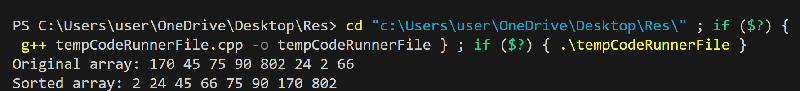

Bucket sort

Bucket sort is a sorting algorithm that separates the input elements into various "buckets" based on their values and then sorts the elements within each bucket separately. It works best when the input numbers are evenly spread across a range.

Bucket sort can be performed in two steps: distribution and collection. The distribution step places elements into their corresponding buckets, and the collection step merges the elements from the buckets to obtain the sorted array.

Example

Let's consider an array of floating-point numbers as our input: [0.42, 0.32, 0.21, 0.91, 0.15, 0.84, 0.67]. We assume that the range of input values is from 0 to 1.
Create an array of empty buckets, where the number of buckets corresponds to the range of input values.
Put each component of the input array into the appropriate bucket as you iterate through the array. The distribution can be done by multiplying the element by the number of buckets and taking the integer part.
Sort the elements within each bucket individually using any suitable sorting algorithm (e.g., insertion sort, quicksort).
Collect the elements from the buckets in order. The elements can be added back into the original array by iterating through the buckets.
The array is now sorted.

Program:

#include <iostream>
#include <vector>
#include <algorithm>

void bucketSort(std::vector<float>& arr) {
    int n = arr.size();

    // Step 1: Create an array of empty buckets
    std::vector<std::vector<float>> buckets(n);

    // Step 2: Distribute elements into buckets
    for (int i = 0; i < n; i++) {
        int bucketIndex = n * arr[i];
        buckets[bucketIndex].push_back(arr[i]);
    }

    // Step 3: Sort elements within each bucket
    for (int i = 0; i < n; i++) {
        std::sort(buckets[i].begin(), buckets[i].end());
    }

    // Step 4: Collect elements from buckets
    int index = 0;
    for (int i = 0; i < n; i++) {
        for (int j = 0; j < buckets[i].size(); j++) {
            arr[index++] = buckets[i][j];
        }
    }
}

int main() {
    std::vector<float> arr = {0.42, 0.32, 0.21, 0.91, 0.15, 0.84, 0.67};

    bucketSort(arr);

    std::cout << "Sorted array: ";
    for (int i = 0; i < arr.size(); i++) {
        std::cout << arr[i] << " ";
    }

    return 0;
}

Explanation:

Create an array of empty buckets, where each bucket represents a range of values.

Put each element in the input array into the appropriate bucket according to its value. The bucket index is determined by multiplying the element by the number of buckets.

Within each bucket, sort the elements. The elements. are sorted in this code using the std::sort function.

Gather the elements. in the proper sequence from the buckets. After going over each bucket iteratively, add the output array's sorted elements.

The main function initializes an input array of floating-point numbers.

Finally, the sorted array is printed.

Program Output: