Time Complexity in Data Structure

Introduction:

Time complexity is a critical concept in computer science and plays a vital role in the design and analysis of efficient algorithms and data structures. It allows us to measure the amount of time an algorithm or data structure takes to execute, which is crucial for understanding its efficiency and scalability.

What is Time Complexity:

Time complexity measures how many operations an algorithm completes in relation to the size of the input. It aids in our analysis of the algorithm's performance scaling with increasing input size. Big O notation (O()) is the notation that is most frequently used to indicate temporal complexity. It offers an upper bound on how quickly an algorithm's execution time will increase.

Best, Worst, and Average Case Complexity:

In analyzing algorithms, we consider three types of time complexity:

Best-case complexity (O(best)): This represents the minimum time required for an algorithm to complete when given the optimal input. It denotes an algorithm operating at its peak efficiency under ideal circumstances.
Worst-case complexity (O(worst)): This denotes the maximum time an algorithm will take to finish for any given input. It represents the scenario where the algorithm encounters the most unfavourable input.
Average-case complexity (O(average)): This estimates the typical running time of an algorithm when averaged over all possible inputs. It provides a more realistic evaluation of an algorithm's performance.

Big O Notation:

Time complexity is frequently expressed using Big O notation. It represents the maximum possible running time for an algorithm given the size of the input. Let's go through some crucial notations.: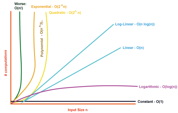

a) O(1) - Constant Time Complexity:

If an algorithm takes the same amount of time to execute no matter how big the input is, it is said to have constant time complexity. This is the best case scenario as it shows how effective the algorithm is. Examples of operations having constant time complexity include accessing a component of an array or executing simple arithmetic calculations.

int constantTimeExample(int arr[], int size) {
    return arr[0];
}

As there is only one operation required to return the first element of the array, the getFirstElement function has an O(1) time complexity.

b) O(log n) - Logarithmic Time Complexity:

According to logarithmic time complexity, the execution time increases logarithmically as the input size increases. Algorithms with this complexity are often associated with efficient searching or dividing problems in half at each step. A well-known illustration of an algorithm having logarithmic time complexity is the binary search.

int binarySearch(int arr[], int size, int target) {


    int low = 0;
    int high = size - 1;


    while (low <= high) {
        int mid = (low + high) / 2;

        if (arr[mid] == target)
            return mid;
        else if (arr[mid] < target)
            low = mid + 1;
        else
            high = mid - 1;
    }

    return -1; // Not found
}

The binarySearch function has a time complexity of O(log n) as it continuously halves the search space until it finds the target element or determines its absence.

c) O(n) - Linear Time Complexity:

According to linear time complexity, the running time grows linearly with the size of the input. When navigating data structures or performing actions on each piece, it is frequently noticed. For example, traversing an array or linked list to find a specific element.

int linearTimeExample(int arr[], int size) {
    int sum = 0;


    for (int i = 0; i < size; i++) {
        sum += arr[i];
    }

    return sum;
}

The printArray function has a time complexity of O(n) as it iterates over each element in the array to print its value.

d) O(n^2) - Quadratic Time Complexity:

An algorithm whose runtime quadratically increases with input size. O(n^2) denotes quadratic time complexity, in which an algorithm's execution time scales quadratically with the amount of the input. This type of time complexity is often observed in algorithms that involve nested iterations or comparisons between multiple elements.

void printPairs(int arr[], int size) {
    for (int i = 0; i < size; i++) {
        for (int j = 0; j < size; j++) {
            cout << "(" << arr[i] << ", " << arr[j] << ") ";
        }
    }
}

The printPairs function has a time complexity of O(n^2) as it performs nested iterations over the array, resulting in a quadratic relationship between the execution time and the input size.

e) O(2^n) - Exponential Time Complexity:

An algorithm that exhibits an exponential relationship between the execution time and the input size. Exponential time complexity indicates that the algorithm's execution time doubles with each additional element in the input, making it highly inefficient for larger input sizes. This type of time complexity is often observed in algorithms that involve an exhaustive search or generate all possible combinations.

int fibonacci(int n) {
    if (n <= 1)
        return n;
    return fibonacci(n - 1) + fibonacci(n - 2);
}

The Fibonacci function has a time complexity of O(2^n) as it recursively calculates the Fibonacci sequence, resulting in an exponential increase in the execution time as the input size increases.

f) O(n!) - Factorial Time Complexity:

An algorithm whose runtime increases proportionally to the size of the input. This kind of time complexity is frequently seen in algorithms that generate every combination or permutation of a set of components.

void permute(string str, int l, int r) {
    if (l == r) {

        cout << str << " ";
        return;
    }
    for (int i = l; i <= r; i++) {
        swap(str[l], str[i]);
        permute(str, l + 1, r);
        swap(str[l], str[i]);
    }
}

The permute function has a time complexity of O(n!) as it generates all possible permutations of a given string, resulting in a factorial increase in the execution time as the input size increases.

How to Calculate Time Complexity?

Analysing the growth rate of an algorithm's running time as input size grows is necessary to determine how time-complex it is. It gives an estimate of how the algorithm performs as the input size increases. Here are the general steps to calculate time complexity:

Identify the algorithm: Determine the specific algorithm or code snippet for which you want to calculate the time complexity. It could consist of a series of operations combined with a loop or a recursive function.
Identify the input size: Identify the elements that make up the algorithm's input size. For example, if the algorithm operates on an array, the input size could be the length of the array.
Determine the basic operations: Identify the fundamental operations that contribute to the running time of the algorithm. These operations could be comparisons, assignments, arithmetic operations, function calls, or any other significant actions.
Count the operations: Analyze how many times each basic operation is executed as a function of the input size. You may need to consider different scenarios or branches within the algorithm.
Express the count as a function of the input size: Create a mathematical expression that represents the count of basic operations as a function of the input size. It ought to outline the worst-case scenario or the performance limit of the algorithm.
Simplify the expression: Simplify the mathematical expression by removing constants, lower-order terms, and insignificant factors. Focus on the most dominant term that represents the growth rate of the algorithm.
Determine the time complexity notation: Use Big O notation to express the condensed expression, where Big O indicates the time complexity's upper bound. O(1) stands for constant time, O(n) for linear time, O(n^2) for quadratic time, and so forth are common notations.

Time Complexity of Different Data Structures:

Here are the time complexities associated with common data structures:

Arrays:

Access: O(1)
Search: O(n)
Insertion (at the end): O(1)
Insertion (at the beginning or middle): O(n)
Deletion (from the end): O(1)
Deletion (from the beginning or middle): O(n)

Linked Lists:

Access: O(n)
Search: O(n)
Insertion (at the beginning): O(1)
Insertion (at the end, with a tail pointer): O(1)
Insertion (at the end, without a tail pointer): O(n)
Insertion (in the middle): O(n)
Deletion (from the beginning): O(1)
Deletion (from the end, with a tail pointer): O(1)
Deletion (from the end, without a tail pointer): O(n)
Deletion (from the middle): O(n)

Doubly Linked List:

Accessing an element by index: O(n)
Searching for an element: O(n)
Insertion (at the beginning): O(1)
Insertion (at the end, with a tail pointer): O(1)
Insertion (at the end, without a tail pointer): O(n)
Insertion (in the middle): O(n)
Deletion (from the beginning): O(1)
Deletion (from the end, with a tail pointer): O(1)
Deletion (from the end, without a tail pointer): O(n)
Deletion (from the middle): O(n)

Stacks:

Push: O(1)
Pop: O(1)
Peek: O(1)

Queues:

Enqueue: O(1)
Dequeue: O(1)
Peek: O(1)

Hash Tables:

Search: O(1) - on average, assuming a good hash function and minimal collisions
Insertion: O(1) - on average, assuming a good hash function and minimal collisions
Deletion: O(1) - on average, assuming a good hash function and minimal collisions

Binary Search Trees (BSTs):

Search: O(log n) - on average for balanced BST, O(n) worst case for unbalanced BST
Insertion: O(log n) - on average for balanced BST, O(n) worst case for unbalanced BST
Deletion: O(log n) - on average for balanced BST, O(n) worst case for unbalanced BST

AVL Tree:

Searching for an element: O(log n)
Insertion of an element: O(log n)
Deletion of an element: O(log n)

B-Tree:

Searching for an element: O(log n)
Insertion of an element: O(log n)
Deletion of an element: O(log n)

Red-Black Tree:

Searching for an element: O(log n)
Insertion of an element: O(log n)
Deletion of an element: O(log n)

Analyzing Algorithms with Time Complexity:

The best algorithm and data structure for a specific task must be chosen, and this requires an understanding of temporal complexity. We can estimate the scalability and performance of our algorithms by looking at time complexity. It enables us to make informed decisions during algorithm design and optimization.

For example, suppose we have a large dataset in which we frequently need to search for specific items. In such cases, a Binary Search Tree (BST) would provide efficient search operations with a time complexity of O(log n). However, if the dataset requires frequent insertions and deletions, a linked list or an array with O(1) insertion and deletion at the beginning may be a better choice.

Conclusion:

In conclusion, understanding time complexity in data structures is crucial for analyzing and evaluating the efficiency and performance of algorithms. Time complexity is a measure of how long an algorithm takes to run as the size of the input increases. It provides valuable insights into how an algorithm scales and helps in making informed decisions about algorithm selection and optimization.

Next TopicArrays are best Data Structure

← prev next →