Check for possible paths in the 2D Matrix

Finding every path from the top-left corner to the bottom-right corner of a 2D matrix is a classic algorithmic problem-solving issue. To effectively walk through the matrix and reveal every possible path, this problem requires investigating a variety of methodologies, such as dynamic programming and backtracking. We will examine many approaches and their descriptions, explanations, and solution codes in this extensive book, along with a time and space complexity analysis.

A 2D matrix can be traversed by backtracking or dynamic programming to locate every path that could exist. Here's a sample of Python code that will find every path from a given matrix's top-left corner to its bottom-right corner by backtracking. For each section of the code, I'll also include some content-style comments.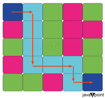

Check for possible paths in the 2D Matrix

Problem Description:

Assume you have a 2D matrix with numerical values in every cell. Finding every possible route from the top-left corner to the bottom-right corner of the matrix is the current task. The objective is to find every route while following the movement restrictions, which limit the movement to only right and down directions.

Approach 1: Backtracking

Description:

Backtracking is a methodical algorithm that builds candidates incrementally to investigate every possible solution to a problem, then goes back when it finds that the current candidate cannot be finished to a workable answer. The backtracking method in our matrix problem entails systematically investigating every possible move-both down and right-until the goal is attained.

Explanation:

The backtracking method investigates two possible moves: right and down, beginning at the top-left corner of the matrix. It keeps track of the current path by repeating this step for every successive cell. When the path reaches the bottom-right corner, it gets added to the list of solutions. The program goes back to the previous cell and investigates the other move if it comes to a dead end.

Solution Code

def find_all_paths(matrix):
    def backtrack(i, j, path):
        if i == rows - 1 and j == cols - 1:
            paths.append(path.copy())
            return

        if j + 1 < cols:
            path.append((i, j + 1))
            backtrack(i, j + 1, path)
            path.pop()

        if i + 1 < rows:
            path.append((i + 1, j))
            backtrack(i + 1, j, path)
            path.pop()

    rows, cols = len(matrix), len(matrix[0])
    paths = []
    backtrack(0, 0, [(0, 0)])
    return paths

Output:

Time Complexity:

The backtracking method has an exponential time complexity, O(2^(m+n)), where m and n are the matrix's dimensions. This is due to the algorithm's worst-case exploration of every potential path.

Space Complexity:

The matrix's dimensions, m and n, determine the space complexity, which is O(m+n). This takes into consideration the space needed for storing the pathways.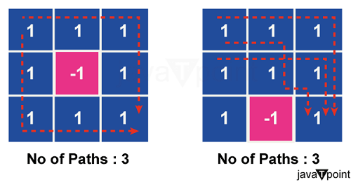

Approach 2: Dynamic Programming

Description:

One method for solving problems by dividing them into smaller, overlapping subproblems is called dynamic programming. To save repeat calculations, it saves the answers to these subproblems. Dynamic programming can be used to effectively locate every path in the context of our matrix problem while preventing needless recalculations.

Explanation:

To store the number of pathways to each cell in the matrix, a 2D array must be created as part of the dynamic programming solution. The algorithm iteratively fills in the array by adding the number of paths from the cell to the left and the cell above, starting from the top-left corner. The total number of unique pathways is shown by the final value in the lower-right corner. A separate stage of backtracking is used to obtain the pathways themselves.

Solution Code:

def fin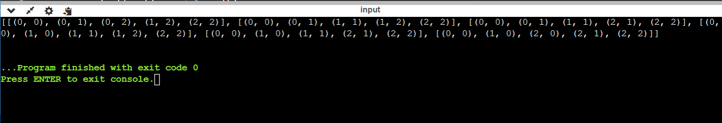d_all_paths_dp(matrix):
    rows, cols = len(matrix), len(matrix[0])

    # Create a 2D array to store the number of paths to each cell
    dp = [[0] * cols for _ in range(rows)]

    # Initialize the top-left corner
    dp[0][0] = 1

    # Fill the first row
    for j in range(1, cols):
        dp[0][j] = 1

    # Fill the first column
    for i in range(1, rows):
        dp[i][0] = 1

    # Fill the rest of the array
    for i in range(1, rows):
        for j in range(1, cols):
            dp[i][j] = dp[i - 1][j] + dp[i][j - 1]

    # Backtrack to retrieve paths
    def backtrack(i, j, path):
        if i == 0 and j == 0:
            paths.append(path[::-1])
            return

        if i - 1 >= 0 and dp[i - 1][j] > 0:
            backtrack(i - 1, j, path + [(i - 1, j)])

        if j - 1 >= 0 and dp[i][j - 1] > 0:
            backtrack(i, j - 1, path + [(i, j - 1)])

    # List to store paths
    paths = []

    # Start backtracking from the bottom-right corner
    backtrack(rows - 1, cols - 1, [(rows - 1, cols - 1)])

    return paths

Output:

Time Complexity:

The dynamic programming solution has an O(m * n) time complexity, where m and n are the matrix's dimensions. This is a result of the algorithm filling the whole array of dp.

Space Complexity:

Because the dp array and the matrix have the same dimensions, the space complexity is thus O(m * n).

Conclusion:

In conclusion, figuring out how to solve the 2D matrix pathfinding problem requires experimenting with different strategies. Backtracking is useful for small matrices with constrained space since it investigates paths iteratively with exponential time complexity. Using a memoization table, dynamic programming, which has polynomial time complexity, optimizes effectively for larger matrices but at the expense of more space.

The decision between them is based on the trade-offs between space and time, which are impacted by the size of the matrix and particular limitations. Comprehending these tactics offers a significant understanding of algorithmic problem-solving, enabling one to make well-informed choices depending on the particular features and demands of the task at hand.

Next TopicFind Triplets with zero-sum

← prev next →