Hash Table

Hash table is one of the most important data structures that uses a special function known as a hash function that maps a given value with a key to access the elements faster.

A Hash table is a data structure that stores some information, and the information has basically two main components, i.e., key and value. The hash table can be implemented with the help of an associative array. The efficiency of mapping depends upon the efficiency of the hash function used for mapping.

For example, suppose the key value is John and the value is the phone number, so when we pass the key value in the hash function shown as below:

Hash(key)= index;

When we pass the key in the hash function, then it gives the index.

Hash(john) = 3;

The above example adds the john at the index 3.

Drawback of Hash function

A Hash function assigns each value with a unique key. Sometimes hash table uses an imperfect hash function that causes a collision because the hash function generates the same key of two different values.

Hashing

Hashing is one of the searching techniques that uses a constant time. The time complexity in hashing is O(1). Till now, we read the two techniques for searching, i.e., linear search and binary search. The worst time complexity in linear search is O(n), and O(logn) in binary search. In both the searching techniques, the searching depends upon the number of elements but we want the technique that takes a constant time. So, hashing technique came that provides a constant time.

In Hashing technique, the hash table and hash function are used. Using the hash function, we can calculate the address at which the value can be stored.

The main idea behind the hashing is to create the (key/value) pairs. If the key is given, then the algorithm computes the index at which the value would be stored. It can be written as:

Index = hash(key)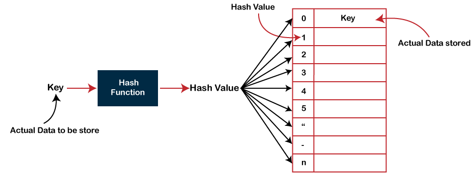

There are three ways of calculating the hash function:

• Division method
• Folding method
• Mid square method

In the division method, the hash function can be defined as:

h(k_i) = k_i % m;

where m is the size of the hash table.

For example, if the key value is 6 and the size of the hash table is 10. When we apply the hash function to key 6 then the index would be:

h(6) = 6%10 = 6

The index is 6 at which the value is stored.

Collision

When the two different values have the same value, then the problem occurs between the two values, known as a collision. In the above example, the value is stored at index 6. If the key value is 26, then the index would be:

h(26) = 26%10 = 6

Therefore, two values are stored at the same index, i.e., 6, and this leads to the collision problem. To resolve these collisions, we have some techniques known as collision techniques.

The following are the collision techniques:

• Open Hashing: It is also known as closed addressing.
• Closed Hashing: It is also known as open addressing.

Open Hashing

In Open Hashing, one of the methods used to resolve the collision is known as a chaining method.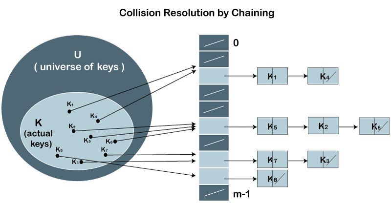

Let's first understand the chaining to resolve the collision.

Suppose we have a list of key values

A = 3, 2, 9, 6, 11, 13, 7, 12 where m = 10, and h(k) = 2k+3

In this case, we cannot directly use h(k) = k_i/m as h(k) = 2k+3

• The index of key value 3 is:

index = h(3) = (2(3)+3)%10 = 9

The value 3 would be stored at the index 9.

• The index of key value 2 is:

index = h(2) = (2(2)+3)%10 = 7

The value 2 would be stored at the index 7.

• The index of key value 9 is:

index = h(9) = (2(9)+3)%10 = 1

The value 9 would be stored at the index 1.

• The index of key value 6 is:

index = h(6) = (2(6)+3)%10 = 5

The value 6 would be stored at the index 5.

• The index of key value 11 is:

index = h(11) = (2(11)+3)%10 = 5

The value 11 would be stored at the index 5. Now, we have two values (6, 11) stored at the same index, i.e., 5. This leads to the collision problem, so we will use the chaining method to avoid the collision. We will create one more list and add the value 11 to this list. After the creation of the new list, the newly created list will be linked to the list having value 6.

• The index of key value 13 is:

index = h(13) = (2(13)+3)%10 = 9

The value 13 would be stored at index 9. Now, we have two values (3, 13) stored at the same index, i.e., 9. This leads to the collision problem, so we will use the chaining method to avoid the collision. We will create one more list and add the value 13 to this list. After the creation of the new list, the newly created list will be linked to the list having value 3.

• The index of key value 7 is:

index = h(7) = (2(7)+3)%10 = 7

The value 7 would be stored at index 7. Now, we have two values (2, 7) stored at the same index, i.e., 7. This leads to the collision problem, so we will use the chaining method to avoid the collision. We will create one more list and add the value 7 to this list. After the creation of the new list, the newly created list will be linked to the list having value 2.

• The index of key value 12 is:

index = h(12) = (2(12)+3)%10 = 7

According to the above calculation, the value 12 must be stored at index 7, but the value 2 exists at index 7. So, we will create a new list and add 12 to the list. The newly created list will be linked to the list having a value 7.

The calculated index value associated with each key value is shown in the below table:

Closed Hashing

In Closed hashing, three techniques are used to resolve the collision:

1. Linear probing
2. Quadratic probing
3. Double Hashing technique

Linear Probing

Linear probing is one of the forms of open addressing. As we know that each cell in the hash table contains a key-value pair, so when the collision occurs by mapping a new key to the cell already occupied by another key, then linear probing technique searches for the closest free locations and adds a new key to that empty cell. In this case, searching is performed sequentially, starting from the position where the collision occurs till the empty cell is not found.

Let's understand the linear probing through an example.

Consider the above example for the linear probing:

A = 3, 2, 9, 6, 11, 13, 7, 12 where m = 10, and h(k) = 2k+3

The key values 3, 2, 9, 6 are stored at the indexes 9, 7, 1, 5 respectively. The calculated index value of 11 is 5 which is already occupied by another key value, i.e., 6. When linear probing is applied, the nearest empty cell to the index 5 is 6; therefore, the value 11 will be added at the index 6.

The next key value is 13. The index value associated with this key value is 9 when hash function is applied. The cell is already filled at index 9. When linear probing is applied, the nearest empty cell to the index 9 is 0; therefore, the value 13 will be added at the index 0.

The next key value is 7. The index value associated with the key value is 7 when hash function is applied. The cell is already filled at index 7. When linear probing is applied, the nearest empty cell to the index 7 is 8; therefore, the value 7 will be added at the index 8.

The next key value is 12. The index value associated with the key value is 7 when hash function is applied. The cell is already filled at index 7. When linear probing is applied, the nearest empty cell to the index 7 is 2; therefore, the value 12 will be added at the index 2.

Quadratic Probing

In case of linear probing, searching is performed linearly. In contrast, quadratic probing is an open addressing technique that uses quadratic polynomial for searching until a empty slot is found.

It can also be defined as that it allows the insertion ki at first free location from (u+i²)%m where i=0 to m-1.

Let's understand the quadratic probing through an example.

Consider the same example which we discussed in the linear probing.

A = 3, 2, 9, 6, 11, 13, 7, 12 where m = 10, and h(k) = 2k+3

The key values 3, 2, 9, 6 are stored at the indexes 9, 7, 1, 5, respectively. We do not need to apply the quadratic probing technique on these key values as there is no occurrence of the collision.

The index value of 11 is 5, but this location is already occupied by the 6. So, we apply the quadratic probing technique.

When i = 0

Index= (5+0²)%10 = 5

When i=1

Index = (5+1²)%10 = 6

Since location 6 is empty, so the value 11 will be added at the index 6.

The next element is 13. When the hash function is applied on 13, then the index value comes out to be 9, which we already discussed in the chaining method. At index 9, the cell is occupied by another value, i.e., 3. So, we will apply the quadratic probing technique to calculate the free location.

When i=0

Index = (9+0²)%10 = 9

When i=1

Index = (9+1²)%10 = 0

Since location 0 is empty, so the value 13 will be added at the index 0.

The next element is 7. When the hash function is applied on 7, then the index value comes out to be 7, which we already discussed in the chaining method. At index 7, the cell is occupied by another value, i.e., 7. So, we will apply the quadratic probing technique to calculate the free location.

When i=0

Index = (7+0²)%10 = 7

When i=1

Index = (7+1²)%10 = 8

Since location 8 is empty, so the value 7 will be added at the index 8.

The next element is 12. When the hash function is applied on 12, then the index value comes out to be 7. When we observe the hash table then we will get to know that the cell at index 7 is already occupied by the value 2. So, we apply the Quadratic probing technique on 12 to determine the free location.

When i=0

Index= (7+0²)%10 = 7

When i=1

Index = (7+1²)%10 = 8

When i=2

Index = (7+2²)%10 = 1

When i=3

Index = (7+3²)%10 = 6

When i=4

Index = (7+4²)%10 = 3

Since the location 3 is empty, so the value 12 would be stored at the index 3.

The final hash table would be: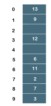

Therefore, the order of the elements is 13, 9, _, 12, _, 6, 11, 2, 7, 3.

Double Hashing

Double hashing is an open addressing technique which is used to avoid the collisions. When the collision occurs then this technique uses the secondary hash of the key. It uses one hash value as an index to move forward until the empty location is found.

In double hashing, two hash functions are used. Suppose h₁(k) is one of the hash functions used to calculate the locations whereas h₂(k) is another hash function. It can be defined as "insert k_i at first free place from (u+v*i)%m where i=(0 to m-1)". In this case, u is the location computed using the hash function and v is equal to (h₂(k)%m).

Consider the same example that we use in quadratic probing.

A = 3, 2, 9, 6, 11, 13, 7, 12 where m = 10, and

h₁(k) = 2k+3

h₂(k) = 3k+1

As we know that no collision would occur while inserting the keys (3, 2, 9, 6), so we will not apply double hashing on these key values.

On inserting the key 11 in a hash table, collision will occur because the calculated index value of 11 is 5 which is already occupied by some another value. Therefore, we will apply the double hashing technique on key 11. When the key value is 11, the value of v is 4.

Now, substituting the values of u and v in (u+v*i)%m

When i=0

Index = (5+4*0)%10 =5

When i=1

Index = (5+4*1)%10 = 9

When i=2

Index = (5+4*2)%10 = 3

Since the location 3 is empty in a hash table; therefore, the key 11 is added at the index 3.

The next element is 13. The calculated index value of 13 is 9 which is already occupied by some another key value. So, we will use double hashing technique to find the free location. The value of v is 0.

Now, substituting the values of u and v in (u+v*i)%m

When i=0

Index = (9+0*0)%10 = 9

We will get 9 value in all the iterations from 0 to m-1 as the value of v is zero. Therefore, we cannot insert 13 into a hash table.

The next element is 7. The calculated index value of 7 is 7 which is already occupied by some another key value. So, we will use double hashing technique to find the free location. The value of v is 2.

Now, substituting the values of u and v in (u+v*i)%m

When i=0

Index = (7 + 2*0)%10 = 7

When i=1

Index = (7+2*1)%10 = 9

When i=2

Index = (7+2*2)%10 = 1

When i=3

Index = (7+2*3)%10 = 3

When i=4

Index = (7+2*4)%10 = 5

When i=5

Index = (7+2*5)%10 = 7

When i=6

Index = (7+2*6)%10 = 9

When i=7

Index = (7+2*7)%10 = 1

When i=8

Index = (7+2*8)%10 = 3

When i=9

Index = (7+2*9)%10 = 5

Since we checked all the cases of i (from 0 to 9), but we do not find suitable place to insert 7. Therefore, key 7 cannot be inserted in a hash table.

The next element is 12. The calculated index value of 12 is 7 which is already occupied by some another key value. So, we will use double hashing technique to find the free location. The value of v is 7.

Now, substituting the values of u and v in (u+v*i)%m

When i=0

Index = (7+7*0)%10 = 7

When i=1

Index = (7+7*1)%10 = 4

Since the location 4 is empty; therefore, the key 12 is inserted at the index 4.

The final hash table would be: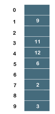

The order of the elements is _, 9, _, 11, 12, 6, _, 2, _, 3.