Compound interest formula in ExcelExcel is usually used for accounting purposes to store the data and perform various types of operations on data. Compound interest formula is one of them that uses the function of Excel to get the result calculated. It is a building block of accounting and the most used formula in banking. Compound interest is advance of simple interest. Simple interest applies only to the principal amount for all years. But the compound interest is applied on both principal amount and interest added to it after a year. In this chapter of the Excel tutorial, we are going to describe the compound interest formula, its usage, and how we could use it on an Excel worksheet. What is the compound interest formula?A simple definition of compound interest is - A compound interest is an interest calculated on interest. Compound interest formula is used to calculate the interest on some amount specified by the user in Excel. Note: For each year principal amount is different for compound interest.Compound interest is a basic building block used in accounting. It calculates the interest on principal amount firstly with some rate of interest for one year and then both principal amount and interest added to it. Understand it with the help of the following diagrammatic representation - 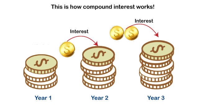
Compound interest is calculated on the initial amount for a year and then interest accumulated with the previous amount. Unlike the simple interest, compound interest takes interest on the amount added with the principal amount after a year. We have two formulas to calculate compound interest, which is discussed in detail in this chapter with examples below:
PrerequisitesThe Excel user must be familiar with some prerequisites, as following below:
Formula of compound interestHere is the general formula to calculate the compound interest. Compound interest formula for single year calculationThis formula of compound interest helps to calculate the interest for a single year only. For example, if you want to calculate the compound interest for three years, you have to calculate interest three times one by one for each year using this formula. Remember that - In each year, the principal amount is different, which is achieved from the calculated compound interest of the previous year. Here, FV = Future value, PV = Present value (This present value refers to Principal amount), r = rate of interest Note: The rate of interest value in percent. So, while using it inside the compound interest formula, use it with its dividend 100. E.g., 12% = 12/100.You can directly put the value to the formula while applying it on the Excel worksheet or provide the respective cell number and apply the compound interest formula. General compound interest formulaThis is another formula to compound interest helps to calculate the interest for any year directly. It is faster than the above one. This formula contains one extra parameter and a math POWER() function. This formula can also be written as =PV*((1+r)^n), where ^ is used for the POWER() function. Here, FV = Future value, PV = Present value (This present value refers to Principal amount), POWER() = It is a power function used in Excel to calculate power for a number. It takes two arguments: number and power. r = rate of interest n = number of years defined by the user for which to calculate interest For example, if you want to calculate the compound interest for eight years, you can use this formula to calculate the for eight years directly in one go. We will define some simple ways to calculate compound interest in Excel. Return ValueThis formula returns the future value (FV), which is used as the principal amount calculating of compound interest. This future value (FV) is a combination of principal amount and interest (calculated through compound interest formula), i.e., FV = principal amount + interest. How to calculate compound interest in Excel?Let's start with a very simple example of calculating the interest on Excel worksheet data. Don't miss even a single step. Thus, you can get confused. We have some data in an Excel worksheet, where initial balance (principal amount) 1000 and the interest rate is 12%. Now, we will calculate the compound interest for 3 years one by one. 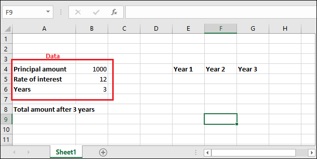
"Rate of interest is always in percent. So, make sure always use 100 in its dividend." 1. Calculate compound interest for each yearFollow each step carefully and don't miss even a single step as you can get confused: Step 1: Go to the cell where to store calculated compound interest and select it. Then in the formula bar, use the following compound interest formula to calculate the interest for the first year. = PV * (1+r) 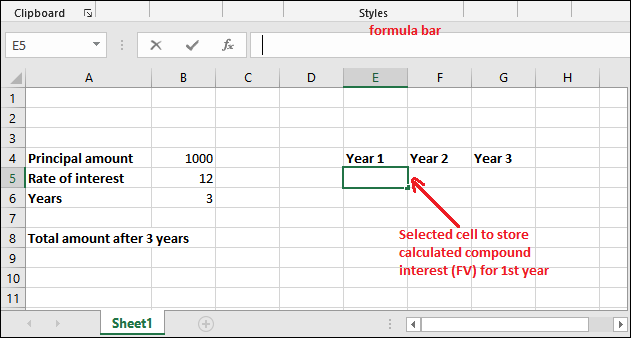
Compound interest for the first year Step 2: Either put the respective values in the formula directly or provide their cell number, which contains respective data. As in the below formula - =B4*(1+B5/100) 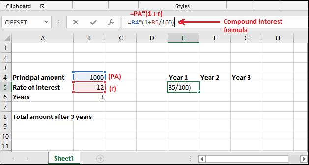
Step 3: Get the calculated compound interest for 1 year in the selected cell by pressing Enter key now. The returned amount is 1120; see the below screenshot. 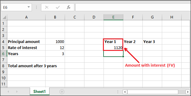
Step 4: If you want to find out the only interest value, subtract the principal amount from the retrieved future value amount (FV), i.e., Interest = Future Value - Principal amount 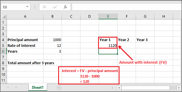
In this way, you can find the interest for every year. But remember that the principal amount and future value always be different for every year. Compound interest for the second year We will now calculate the compound interest for the next year (second year) with the newly retrieved principal amount. For this time, the principal amount is 1120(stored in E5 cell), not 1000. Step 1: Select a cell to keep the newly calculated compound interest amount and write the compound interest for the second year. = PV * (1+r) 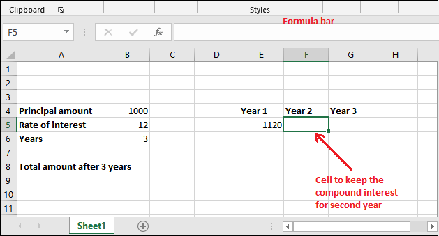
Step 2: Put the following compound interest formula in the formula bar of Excel. =E5*(1+B5/100) 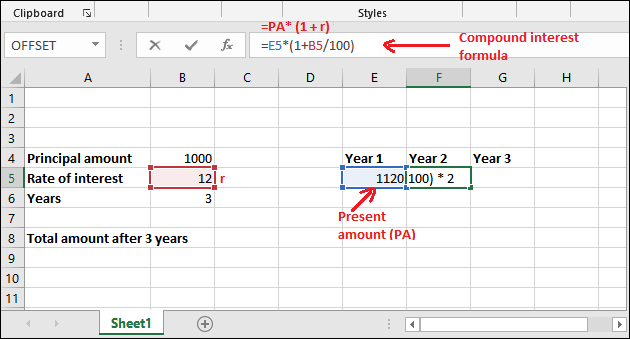
Step 3: Get the calculated compound interest for the 2nd year in the selected cell by pressing Enter key now. The returned amount is 1254.4; see the below screenshot. 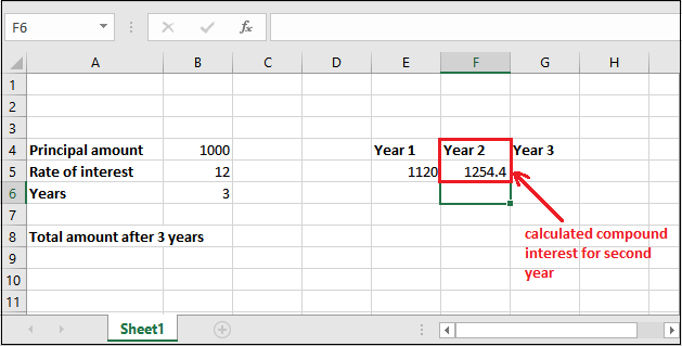
Compound interest for the third year We will now calculate the compound interest for the third year with a new retrieved amount (1254.4). So, the principal amount will be 1254.4 this time, which is stored in the F5 cell. Step 1: Put the following compound interest formula in the formula bar of Excel. =F5*(1+B5/100) 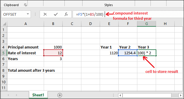
Step 2: Get the calculated compound interest for 3rd year in the selected cell by pressing Enter key now. The returned amount is 1404.928; see the below screenshot. 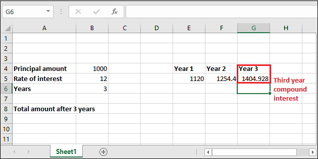
Similarly, you can calculate the compound interest for the other years. 2. General formula to calculate compound interestIn this example, we are going to use this = PV * POWER((1+r), n) formula of compound interest. Follow each step carefully and don't miss even a single step as you can get confused: Step 1: Go to the cell where to store calculated compound interest and select it. Then in the formula bar, use the following compound interest formula to calculate the interest for the first year. = PV * POWER((1+r), n) Step 2: Like the above example, either you can provide the reference of the cell for the respective value needed or directly enter the value for calculation. We are using cell reference. So, our formula will be like, =B4*POWER((1+B5/100), B6) 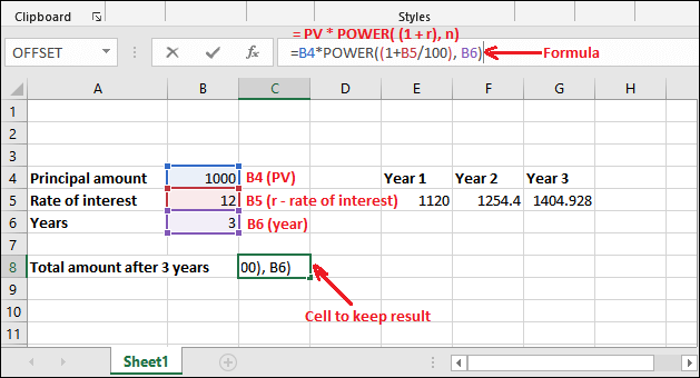
Step 3: Press Enter and get the total amount after calculating three years compound interest in one go. You can see that returned value is 1404.928 after applying compound interest 3 years. 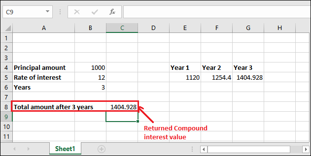
You can also compare both results of compound interest calculated through the different formulas and note that the results are identical. 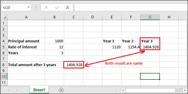
Compounding period per year (monthly, quarterly, annually)Besides the above examples, we have one more example of compound interest. It is a bit different than the above ones. For this example, we have added one more term with the data, i.e., compounding period per year. This term refers to how many times interest given to the user in a year. This compounding period can be monthly, quarterly, semi-year, annually, or whatever you will define while providing data. Let's understand using a real scenario: For example, as we all know, the bank provides compound interest for saving their money in banks. A bank gives interest thrice a year on a quarterly basis. According to this example, the value of compounding period per year will be 3. Formula for this type of compound interest Everything is same as the above formula. Here, p is the period per year. Instead of using the POWER() function, you can write this formula as well - Example 3Steps to calculate quarterly CI for three years Now, let's implement this example practically on Excel worksheet data and understand how this calculation takes place. Step 1: Go to the cell where to store calculated compound interest and select it. Then in the formula bar, use the following compound interest formula to calculate the interest for the first year. = PV * POWER((1+r), n*p) 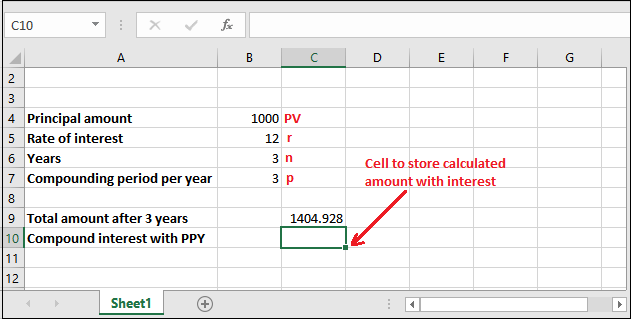
Step 2: Like the above example, either you can provide the reference of the cell for the respective value needed or directly enter the value for calculation. We are using cell reference. So, our formula will be like, =B4*POWER((1+B5/100), B6*B7) 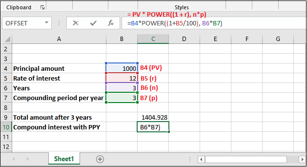
Step 3: Press Enter and see the calculated compound interest returned by Excel, which is 2773.079. 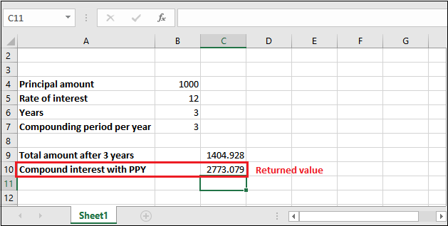
Understand compound interest in the simplest language or term, i.e., "Interest over interest". FV() function and compound interestAll the methods that we have discussed above are manual. It means the user must know the compound interest formula and know its basic terms and usage. If the user has good knowledge of compound interest and its formulas, he/she can easily use it without wasting any time. Although we have provided a detailed description of compound interest and calculation in Excel but if the user still not getting this, we have one more solution. Excel offers FV() function, which is an in-built Excel function used to calculate compound interest. FV() functionFV() refers to the Future Value. It is a built-in function of Excel that is used to calculate the compound interest on some value. Similar to the above methods, it also calculates the future value on investment. It takes five arguments in which the last two are optional. Firstly, see the syntax then we will talk about its parameters. SyntaxEach parameter belongs to a specific value, such as - rate (required) - The rate parameter contains the interest rate to be applied to an amount for each period. nper (required) - It contains the number of compounding periods per year. The compounding period means how many times interest given to the user in a year. It can be monthly, quarterly, or annually. pmt (required) - The pmt is an additional amount per period. It is represented as a negative number. It means that the value must be a negative number. If there is no value in pmt, then put 0 as its value. pv (optional) - Pv refers to the principal investment, which is an optional parameter value. Like the pmt, if there is no value in pv, put 0 as its value. type (optional) - When payments are due. It is also an optional argument whose default value is 0. Here, 0 stands for end of the period and 1 for beginning of the period. Return valueThe FV() function of Excel returns the future value of an investment. ExampleLet's take an example and understand how FV() function works with its parameters. Before we will define a simple scenario: We have deposited 3000 rupees for 4 years at 7% of the annual interest rate compounded monthly. This means compounding period is monthly, i.e., 12 here. There is no additional payment. See the dataset below: 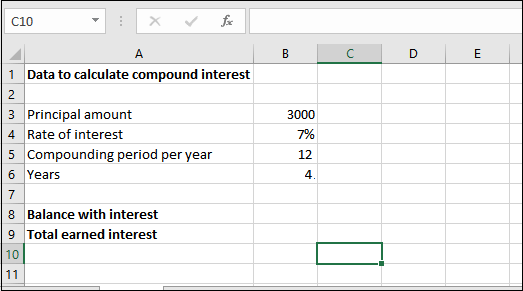
Now, see the detailed explanation;
Hence, the FV() formula goes like - =FV(0.007/12, 4*12, -3000) You can also replace these values with cell reference of the Excel worksheet. =FV(B4/B5, B6*B5, -B3) Step 1: Select the cell to keep the calculated result and write the created FV() formula in the formula bar. 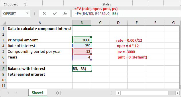
Step 2: Get the Balance returned with interest by pressing the Enter key. See that the returned amount is 3966.16. 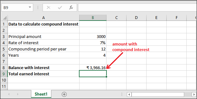
Step 3: You can extract only the compound interest from the amount returned for 4 years and the monthly compounding period. See the result: 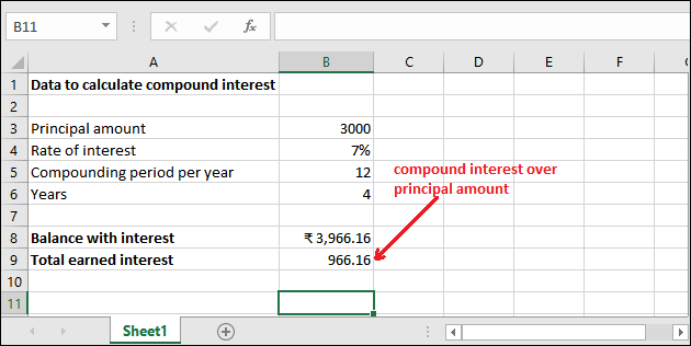
Similarly, you can count the compound interest for other data. Hope you have understood completely how compound interest can be calculated in Excel using manual calculation or using in-built formula.
Next TopicExcel password remover
|
 For Videos Join Our Youtube Channel: Join Now
Feedback
- Send your Feedback to [email protected]
Help Others, Please Share


