| |

VLOOKUP to compare two columns in Microsoft Excel for common values and missing dataWhen we are having the data in two different lists, we may often need to compare them to see what type of information is missing in one of the lists or what type of data is usually present in both lists (that means common data). And one can perform the comparison in various ways which are available in the Excel and the methods which will be used by an individual will depend upon the outcomes (which one wants). In this tutorial, we will discover the various concepts which are as follows:
How can we make a comparison between two columns in Microsoft Excel with the help of the VLOOKUP formula?It was the scenarios, in which we are having two data columns, and we want to figure out which data points from one list primarily exist in the other list, and to achieve this we can make use of the "VLOOKUP" function in order to compare the list to obtain the common values. And if we want to build a "VLOOKUP" formula in its basic form, then we need to perform the following things:
Let us assume that we have the names of the participants present in column "A", say List 1, and the names of those participants who have passed through the qualification rounds present in column "B", say List 2. We want to compare these 2 list to determine which of the participants from Group A has made their way to get enrolled on the main event. To achieve this, we will be making use of the below-mentioned formula: FORMULA: And the above respective formula will be entered into the cell E2. After that, we will drag it down through the cells containing the items in List 1. The table_array is primarily locked with the absolute references ($ C $ 2: $ C $ 9), so it remains constant when copying out the formula to the below individual cells. Now we are encountered with the excel sheet in which the names of the qualified athletes are depicted in column E. And for the rest of the remaining participants, a #N/A error primarily gets appears, which means that their names are not associated with List 2: 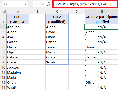
Disguise #N/A errors in Excel sheet The VLOOKUP formula, which we discussed above with the help of the examples basically fulfills its primary objective efficiently, which means returning the shared values and identifying the missing data points in the individual used sheets. Moreover, they also deliver a bunch of #N/A errors that might confused an inexperienced user and make them think that they have committed some mistakes while creating the formula. And to replace the #N/A errors with the respective blank cells, so making use of the VLOOKUP formula in combination with the "IFNA" Or the "IFERROR" function: FORMULA: 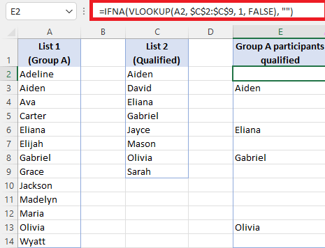
It was well known that our improved formula will return an empty string ("") instead of returning a #N/A error, we can also return our custom text like "Not available in List 2", "Not present in List", or "Not in List 2".
This is considered as the basic VLOOKUP formula that can be used to compare the two columns in Microsoft Excel, depending on our particular task. How to compare two columns in different Microsoft Excel sheets with the help of the VLOOKUP?In real life, the particular columns we need to compare are sometimes present on different sheets. And in a small dataset, we can spot the differences manually by just viewing the two sheets side by side. And to search for it in the other worksheet with the formulas we have to make use of the external reference. And the best practice is to type the formula in our main sheet and switch to the different worksheets, selecting the list with the mouse. Let us Assume that we have List 1 in column A on Sheet1and list 2 in column A on Sheet2, and we can compare the two columns and can find matches with the help of the below-mentioned formula: 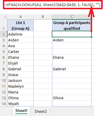
How we can compare two columns and return a common value?In the above examples, we discussed the VLOOKUP formula in its simplest form: And the outcome of the above formula is a list of values that primarily exist in both columns and the blank cells in place of the values that are not available in the second column. For the purpose of getting a list of the common values without gaps, we will be adding the auto-filter to the resulting column and also filtering out the blanks. 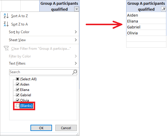
In Microsoft Excel for Microsoft 365 and Excel 2021, which supports dynamic arrays, we can use the "FILTER" function to dynamically shift out the respective blanks. And for this, we will be utilizing the IFNA VLOOKUP formula as the criteria for FILTER: And we should pay much attention that in this case, we must supply the whole List 1 (A2:A14) to the lookup_value argument of the VLOOKUP. The function makes comparison in each lookup value against List 2 (C2:C9) and gives an array of matches and the #N/A errors representing the missing values. The IFNA function usually replaces the errors with the empty strings, and it serves the results to the FILTER function that filters out the blanks (<>"") and outputs an array of matches as the final result effectively: 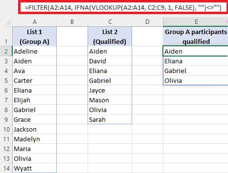
How can we compare the two columns as well as a finding of the missing values? Now to make comparisons of the two columns in Microsoft Excel to find the difference or the missing value, we can proceed with the following methods:
The complete formula will usually take this form: To get rid of the blanks, we will be applying Microsoft Excel's Filter: 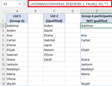
How to identify matches and differences between the two columns in Microsoft Excel?Now if in case we basically wants to add text labels to the first list which indicates that the values are available in the second list and which are not available in the list, so we will make use of the VLOOKUP formula together with the IF and ISNA/ISERROR functions.
Here, the ISNA function catches the #N/A errors generated by VLOOKUP and will pass that intermediate result to the IF function to return the specified text for the mistakes and the other text for successful lookups. And in this example, we have used the labels that are "Not qualified" or "Qualified" labels which are suited for our selected dataset. It can be replaced replace with "Not present in List 2"or "In List 2. The above formula can be efficiently inserted in a column adjacent to List 1 and copied through the various cells which are containing the items in our selected list. 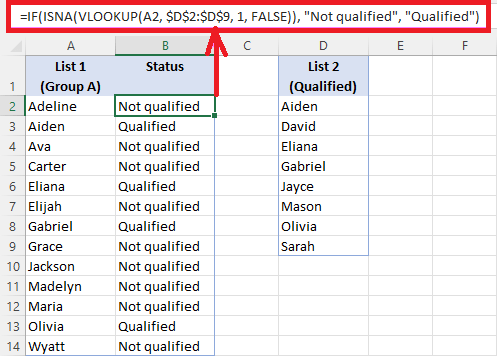
And the other essential methods can be used to identify the matches and the differences in 2 columns with the help of the "MATCH" function. 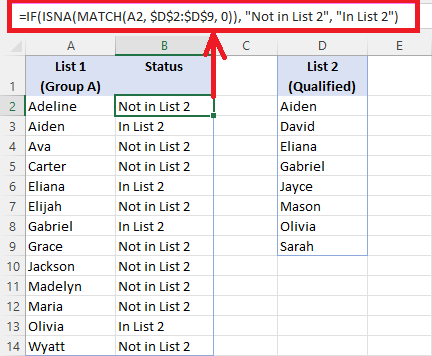
Next TopicDynamic Named Range
|
 For Videos Join Our Youtube Channel: Join Now
Feedback
- Send your Feedback to [email protected]
Help Others, Please Share


