How can one insert Subscript and Superscript in Microsoft Excel

Intro to Subscript in Microsoft Excel

We all know that the particular "Subscript" function n Microsoft Excel is basically used for the purpose of putting the number as well as the text in small fonts on the base of the numbers or on the text effectively.

Furthermore, mathematically it is primarily used very rarely; and we have used such a thing in Chemistry wherein the chemical formulae give the atomic values at the base of any respective alphabet, such as H20, SO2, etc. And this is usually used in the mathematics for the Algorithm where we give such numbers to the bottom of any base numbers respectively.

And the Subscript can be used by right-clicking on the menu's Format Cells option, and then we will be moving to the Font tab by clicking on Subscript to use it wisely.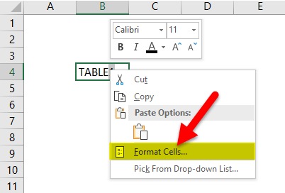

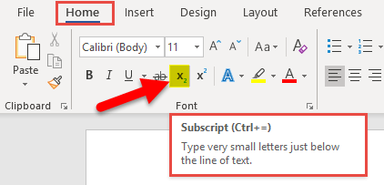
1. The Microsoft Excel data can be formatted differently, and the two basic formats are the Subscript and Superscript formats.
2. The Subscript, as well as the Superscript formats, can be commonly used in MS Word as well as in PowerPoint documents.
3. It is primarily used in the mathematical formula, algebraic expressions & equations that mean writing the number base value OR bases like 49₇. In contrast, in chemistry this could be used in the specification of the chemical substance or the compounds, that is, the chemical formulas like butane C₂H_5,C₆H_6,NO₂, and various other formulas used in the field of chemistry. These mathematical & chemical equations require a Subscript format for a better visual appearance.
4. And the Subscript can also be used for the purpose of differentiating the different types of subatomic particles, i.e. electron, muon, as well as the tau neutrinos that are denoted as ?_e, ?_?and ?_?.
5. The respective subscript format is an easy-to-use function & very simple. The Subscript format can also be applied by the help of the VBA (Virtual Basic for Application) code.

Definition

Subscript:It is considered the small character or the string that usually fits or sits just below the given line of text.

• For example: The appearance of the Subscript format: TABLE₁

This is smaller than the normal text value and has visibility below the baseline.

The shortcut key, as well as the keyboard shortcut for a Subscript format available in Microsoft Excel

We can easily carry out by just making use of a couple of the keys combination that is as follows: Ctrl+1 and then will be pressing Alt+B, and after that we will be then clicking on the "Enter" button.

And the above shortcut key is not pressed out simultaneously; the below-mentioned process does it effectively.

1. One of the initial steps is to select one or more characters we primarily want to format.
2. And then, we will be pressing the Ctrl+ 1 in order to open the Format Cells dialogue box.
3. And once the Format Cells dialogue box appears, we will press the shortcut button that is Alt+B to select the Subscript.
4. In the final step, we will be hitting the "Enter key" to apply the formatting as well as closing of the dialogue box.

How can we add a subscript icon to Quick Access Toolbar?

In the Excel 2016 version, we have an option which can be primarily used for the purpose of adding the Subscript buttons to Quick Access Toolbar as well.

And to set up this, we need to follow the below-mentioned steps which are as follows:

Step 1: First of all, we need to click on the dropdown arrow next to the Quick Access Toolbar present on the left corner of the Excel window and will selecting out the More commands options from the popup menu as well.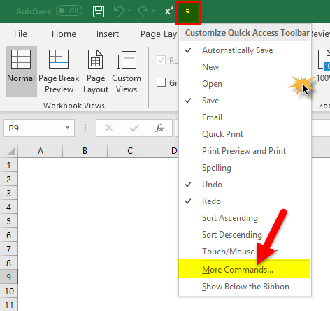

Step 2: After that, the Excel options popup window appears on the screen. And under the choose commands from the select Commands Not in the Ribbon which is under a drop down, we will be selecting the Subscript in the list of commands, and we will click on the Add button respectively: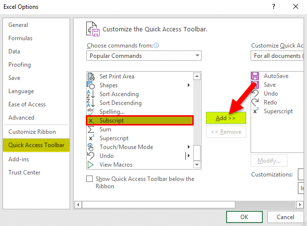

Step 3: In these steps we will be clicking on the "OK" option in order to save our changes as well: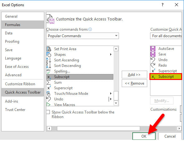

And once we applied all the steps mentioned above one by one, we could see the desired change in the Quick Access Toolbar button, which are present at the top left corner, where it enables us to make use of the subscript format in Microsoft Excel 2016 version with a single key option respectively.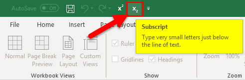

How can one make use of the Subscriptin Microsoft Excel?

It was termed that the Subscript Function is quite simple and easy to use in Microsoft Excel, now we will be seeing how to make use of the Subscript Function in Excel sheet by making use of the various examples.

# Example 1: How one can apply Subscript Format to the Specific alphabet or the word or character in a respective cell

In accordance to the below-mentioned cell, that is cell "B4 is containing the text value which is none other than the TABLE1.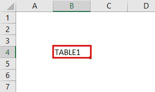

And here in this particular text value, only for the given last alphabet that is 1, we need to apply a SUBSCRIPT format to 1.

Step 1: In the very first step, we will be clicking on cell "B4" and then will press the F2 key so that the text value in cell B4 text gets into the edit mode as well.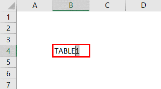

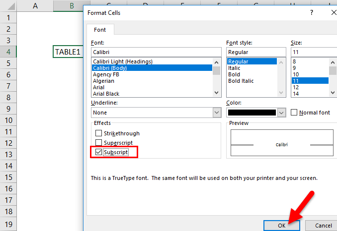
Step 2: In the mouse, we will select only the last alphabet, that is, 1.

After that, we will be opening out a format cell dialogue box by just clicking or pressing the ctrl+1 or right-clicking in the mouse and then selecting the format cells option in it respectively:

Step 3: Now, in the open Format Cells dialogue box, under the Font tab we will be selecting the Subscript under Effects as well:

Step 4: And last, we will click on the"OK"option to save the changes made and close the dialogue box effectively: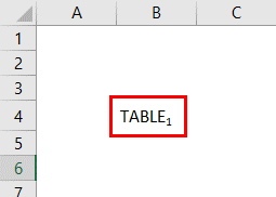

After performing all the steps mentioned earlier, the selected alphabet 1 will be subscripted in cell "B4."

And here are the visual changes or the representation that can be seen in the text value of a cell, i.e. TABLE_1.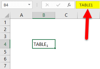

# Example 2: How can we Apply Subscript Format to the whole cell text in an Excel sheet

The below-mentioned cell, "B16", contains the word or the text value that is the 'Electron.'

Here in the text value, we need to apply a Subscript format to the entire cell text respectively: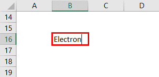

Step 1: First, we will click on cell "B16" and press the F2 key so that the text value in cell B16 text gets into the edit mode.

Step 2: We will select the complete text with the mouse.

After that, we will open a format cell dialogue box by just clicking or pressing the ctrl+1 or right-clicking in the mouse and then will select the format cells option in it as well: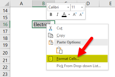

Step 3: And now in the Format Cells dialogue box, under the Font tab, we will be selecting the Subscript option under Effects.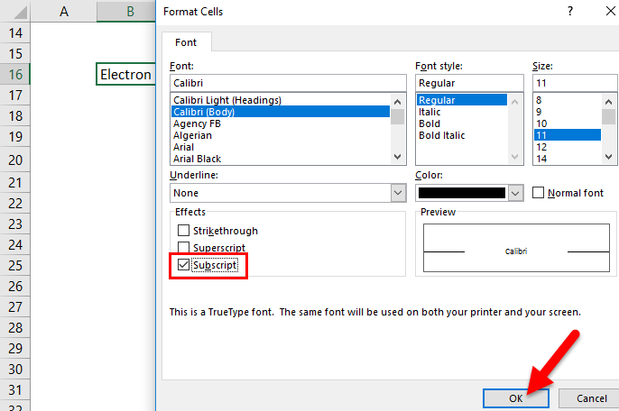

Step 4: And in last, we will click on the"OK"option to save the changes made and close the dialogue box effectively: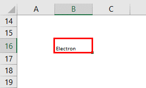

After performing the above steps, we can see that the whole text in cell "B16" will get converted to a subscript format effectively.

And here are the visual changes or the representation that can be seen in the text value of a cell: _Electron.

How to Remove the Superscript Format in a cell

1. For the purpose of removing the superscripts, we need to select the cell format; in the respective Format Cells dialogue box, under the Font tab, uncheck or untick the Subscript option.
2. Moreover, there is no option in Microsoft Excel, nor does it provide any shortcuts or character codes to insert subscripted text or numbers.
3. The subscript option can also be applied to a particular numeric value.

What do you mean by Superscript in Microsoft Excel?

The Superscript in Microsoft Excel is basically used for the purpose of putting the number as well as the text in small fonts which are present just above the base numbers and text. And it is much similar to giving power rose to any base number.

Furthermore, it likes using of the Superscript in order to write the text in the square of base units as well as the text such as: Feet2, Meter2, etc. Similarly, we can also use superscript numbers such as 102 or 25. Superscript is not a function in excel, and it is mainly made for MS Work which deals with text effectively. And in order to activate the Superscript in Excel, we must need to go to the edit mode of the selected cell and then we will be selecting the Format Cells from the right-click menu as well. And from there, we can also tick Superscript from the Fonts tab.

Various examples of Superscripts

Y³, C^f, 3^rd, cos² (30)

• Y³: Here in these, the Superscript is '3', a number for its previous character Y.
• C ^f: Here in these, the Superscript is 'b', a primary character for its previous character C.
• 3^rd: Here in these, the Superscript is 'rd', a string for its previous number 3.
• Cos² (30): In these, the Superscript is '2', a number for its previous string 'cos' respectively.

Hoping that we all understand what Superscript is, so let us begin with how to do it in Microsoft Excel.

Steps that can be used get a Superscript Text in Microsoft Excel

Inputting of the superscript text in Microsoft Excel is a very easy task as compared to others.

• For example, Input X2.

Step 1: First, we will input X2 in any particular cell where we require the Superscript. Now, after that, we will be selecting the number 2 alone by just clicking on F2 and selecting 2: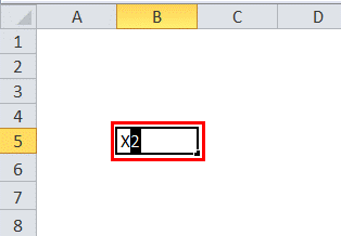

Step 2: And once we select the number 2, we will right-click on the mouse, and a popup will come effectively: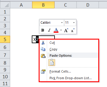

Step 3: And from the popup menu, we will be selecting the Format cells as well: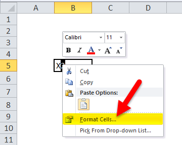

Step 4: The "format cells" menu appears on the screen.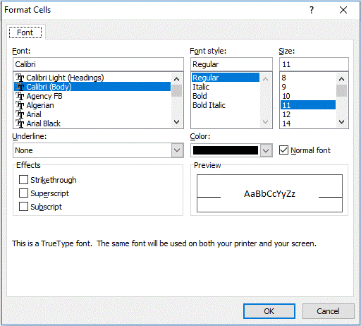

Step 5: And from the menu "Font", we will select the required font for the Superscript effectively: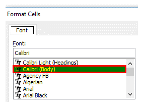

Step 6: And now, from the menu "Font style" and menu "Size", we will be selecting the required font style for the Superscript, such as Italic, bold, as well as the required Size etc.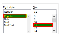

Step 6: After that, from the menu "Effects", we will also select the option superscript.

Step 7: Once we have made selection of the Superscript, we will be then selecting "ok", and just after that we will be able find the number 2 present above the letter X.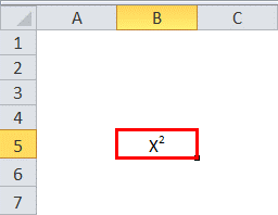

How can one make use of the Superscript in Microsoft Excel?

This Superscript, as well as the subscript feature, is very helpful while working with mathematical and scientifically related data. And we have more ways that are much more beneficial to input superscript text in Microsoft excel.

# Example 1: Superscript in Excel; through the Quick access toolbar

We can now easily input out Superscript by using the QCT. Here are the steps that can be used to achieve this.

Below is the screenshot for the people who need to be made aware of the quick access toolbar.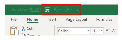

And, we are having an option like as: "Save", "Undo", and "Redo"; hence we need to add the "Superscript" option to QCT.

Step 1: First, we will click on the "File" menu, and the following dropdown menu will appear on the screen. From that dropdown menu, we will be selecting "Options".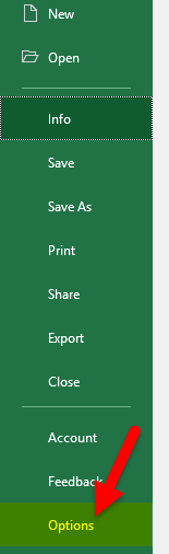

Steps 2: And when we click on "Options", another screen will get appear on the screen: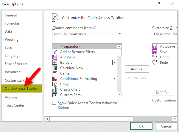

Step 3: Now, From the above screen, we will select the "Quick Access Toolbar" that is effectively highlighted on the left-hand side. And it could be observe that the multiple numbers of commands are visually available on the rectangle screen as well.

And one can easily scroll, as well as select the required commands and then will click on "Add" to add to the QCT as we need the Superscript command; search for that; we will choose the Superscript and click on Add option as well.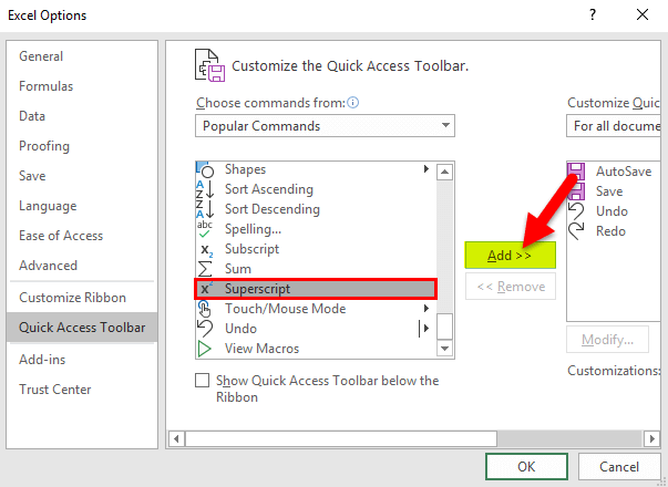

Step 4: And once we are clicking on the "add", the Superscript will move from the left to right side QCT rectangular box.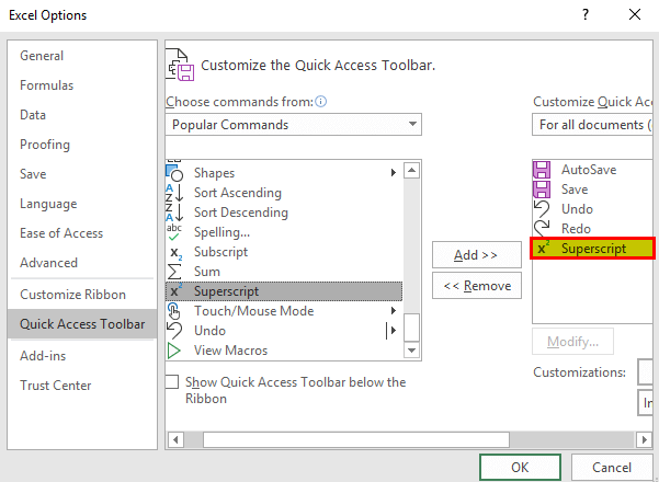

Step 5: After that, we will be clicking on the "Ok" button at the bottom, and the menu will close and return to Microsoft Excel.

Now we can observe the QCT, as there is an additional option visible that is x²marked in the picture respectively: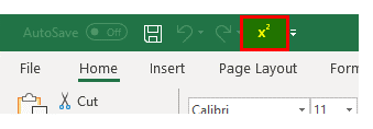

Moreover, it is much easy to input Superscript; we need to select the letter as well as the text we want to convert as Superscript and then click on the X²option in the Quick access toolbar.

And if in case we want to remove the Superscript, and reselect the X²command, then it will be converted to the normal text again.

Example 2: How to apply the Superscript for a given number

Whatever the respective process we have discussed will not work for numbers that mean 2⁵. And we can try this in both ways, either from QAT or right-click, and the movements we move from the cell will also be converted into normal numbers.

Now to apply the Superscript for the given numbers, we need to follow the below-mentioned steps.

Step 1: In these step, we will be clicking on the "Insert" option at the top of the sheet. And if we observe the right-hand side, we can see the option" Equation" as well: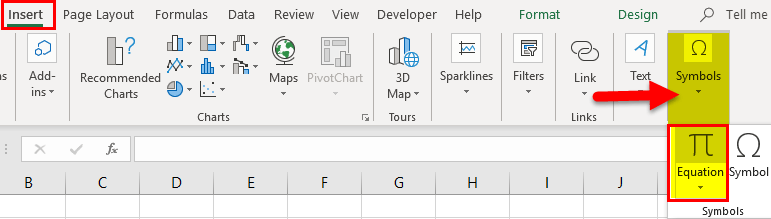

Step 2: Then we will be clicking on the option "Equation", and the menu will get changes to design respectively.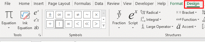

Step 3: After that, we will click on the "e^x" option and mark them. The dropdown option will come from that dropdown, and we will select the format for Superscript.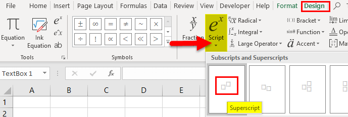

Step 4: And we can observe a pattern in the given cell, as shown: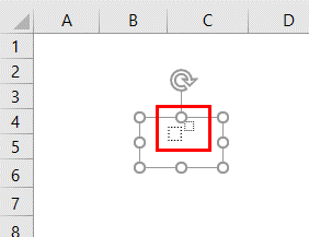

Step 5: Then we will select the first cell, give the Base number, and select the small box at the top to provide the power.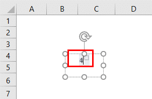

# Example 3: Superscript in Microsoft Excel

And the other way is when we efficiently click on the "Equation", as it will take us to the "design" menu on the left-hand side, we can observe the availability of the "Ink Equation" option in the respective sheet: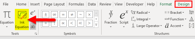

Once we click on "Ink Equation", the other screen will pop up there; and we can write the required text manually by making use of our mouse. And once our text is over, we will be effectively clicking on the "Insert" option available at the bottom of the box effectively.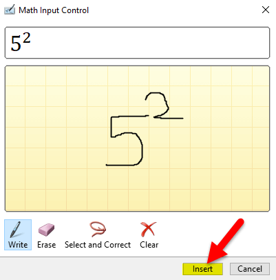

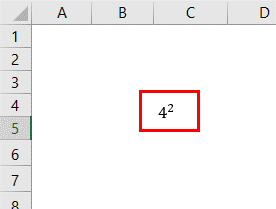
And the outcome for the above is as follows: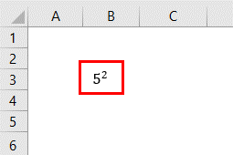

What are the basic things that need to be remembered in Microsoft Excel?

The important things that need to be remembered while working on the insertion of the Subscript as well as the Superscript in an excel sheet by an individual are as follows:

1. Before the Microsoft Excel version 2016, in the Version of EXCEL 2007, EXCEL 2010 and EXCEL 2013, there was no proper subscript button option to format text as a subscript respectively quickly.
   
2. And before applying the subscript format, an individual must convert the given cell to text values containing a formula or any number.
3. Moreover, the Superscript is extensively used in Microsoft excel when an individual is taking mathematical and scientific data input. Superscripts can be input in multiple ways, but those ways are not suitable for a number format. So it is recommended to use the special process for numbers alone.