How to insert a tick symbol and cross mark in Excel

Tick and cross mark symbols are a great control that helps the user to select or deselect an option. Tick marks are also known as a checkbox or check symbol. There are two types of checkmarks in Microsoft Excel - interactive checkbox and tick symbol.

This tutorial we will cover the various methods to insert a tick symbol and cross mark in your Excel worksheets. Following are the methods:

1. Add tick symbol using Excel symbol command
2. Steps to insert tick mark symbol using Excel Formulas
3. Insert checkmark by typing a character code
4. Steps to add tick symbol using Excel keyboard shortcuts
5. Insert the tick symbol automatically in Excel
6. Steps to insert the checkmark as an image
7. Conditional formatting on the basis of tick & cross symbol
8. Points to Remember- Tick and Cross Symbol

What are Tick or cross Symbols?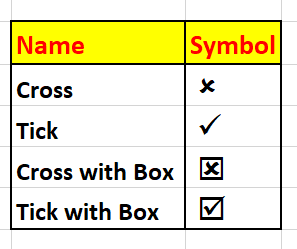

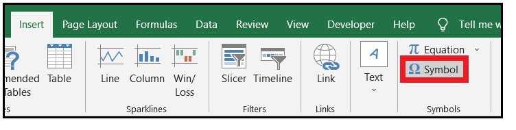
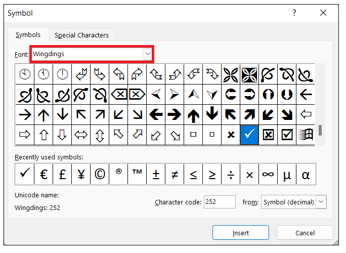
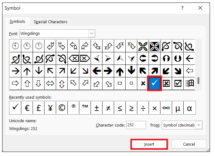
"A tick or cross symbols, also commonly known as check symbol or check mark, is a special too (?) that can be entered in an Excel cell (either in an empty cell or can be inserted as a part of the cell contents). It is used to express the concept of yes or no. For instance, if you want to choose any option you can opt for tick symbol or if you want to say no you can add the cross symbol."

Microsoft Excel provides different methods to insert the checkmark in Excel, and moving ahead we will the detailed steps of each of the techniques.

All of the methods covered in this tutorial are quick, easy, and work for all versions of Microsoft Excel. Let's move ahead with the different methods to add the checkmark or tick symbol in your Excel worksheet.

How to put a tick in Excel using the Symbol command

Symbol command is one of the most commonly used methods to add the tick symbol in your Excel worksheet. Let's have a look at the steps to incorporate this:

1. The first step is to select a cell in your worksheet where you want to add the tick symbol. In our case we have selected cell B5.
   
2. From the Excel ribbon menu, click on the Insert tab > Symbols group, and select the Symbol option.
   
3. As shown the Symbol dialog window will appear. Go to the Symbols tab, click on the drop-down arrow present next to the Font box, and from the options select the Wingdings.
   
4. It will show a list of checkmark and cross symbols at the bottom of the window list. Select the tick symbol (or any other of your likings), and click on the Insert button.
   
5. Once done, click on the Close option to close the Symbol dialog box. The tick symbol will be inserted at the selected position.
   

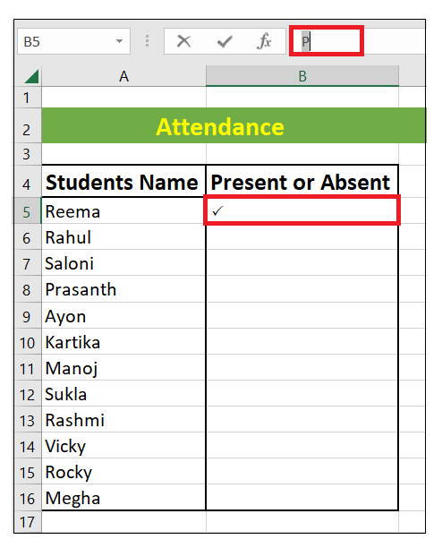
NOTE: As soon as you've selected a particular symbol in the Symbol dialogue window, Excel will show its code in the Character code box at the bottom. For example, the character code of the tick symbol (?) is 252 (refer to the above image). Remember this code, as it will help you to quickly write a formula and insert the tick or cross marks in the selected cell (which will cover in the next section).

1. Using the Symbol method, you can add the tick mark or cross mark symbols anywhere in your worksheet i.e., in an empty cell or can insert it as a part of the cell contents.

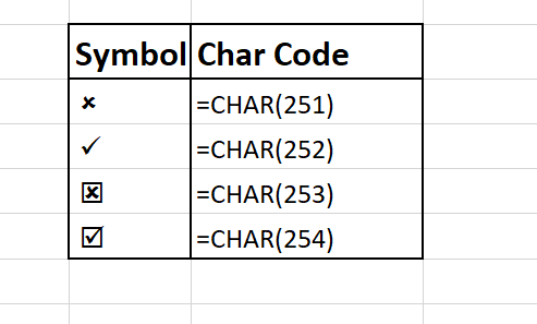
Steps to insert tick mark symbol using Excel Formulas

Though many users may find this method challenging as one needs to remember the special character codes, if you are an Excel expert and love working with formulas, you may be looking for this method.

NOTE: Inserting a tick mark using the Char function will only work for an empty cell.

Before moving ahead with the steps, let's have a look at the table of different symbols codes:

To put the symbol formula in your Excel formula, perform the following steps:

1. Select an empty cell, in our case we have selected B5 cell.
   
2. Select the wingdings font from the symbol dialog window. Put the below formula in the selected cell.
   =CHAR(252) or =CHAR(254)
3. If you want to insert a cross symbol you can put the following character code.
   =CHAR(251) or =CHAR(253)

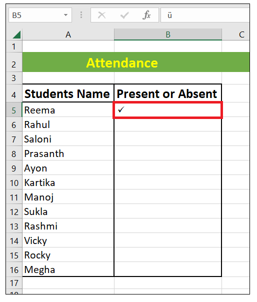
As a result, it will quickly insert the symbols in your Excel worksheet.

Refer to the below screenshot.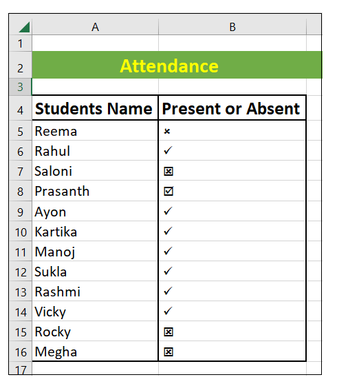

Steps to add tick symbol using Excel keyboard shortcuts

Another quick method to add a tick or cross symbol in your Excel worksheets is using keyboard shortcuts. You can also use this method if you don't like the appearance of the symbols that we have inserted above in this tutorial. The keyboard shortcuts will give you more variations. The following table shows the different shortcuts for tick and cross symbols.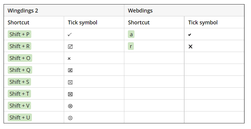

Perform the following steps to implement this method:

1. Select an empty cell, in our case we have selected B5.
2. From the symbols dialogue window, select wingdings font from the required cells. Press any corresponding keyboard shortcuts (you can insert either Wingdings 2 or Webdings) that you want to apply in the selected cells.
3. You will have the resulting output.

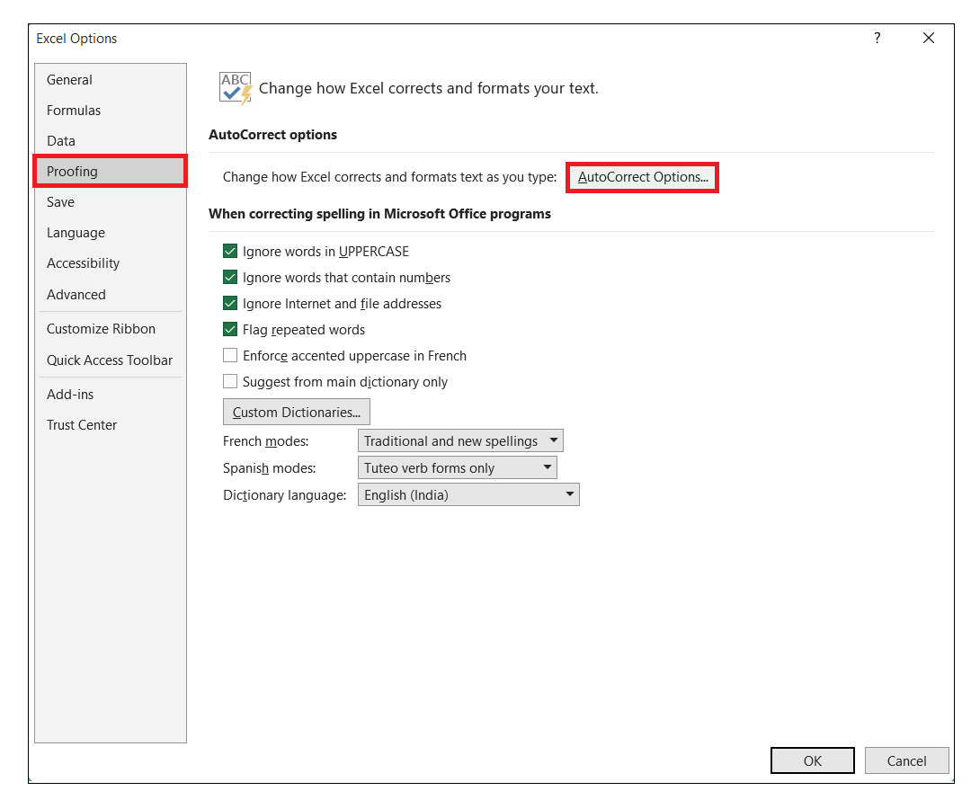
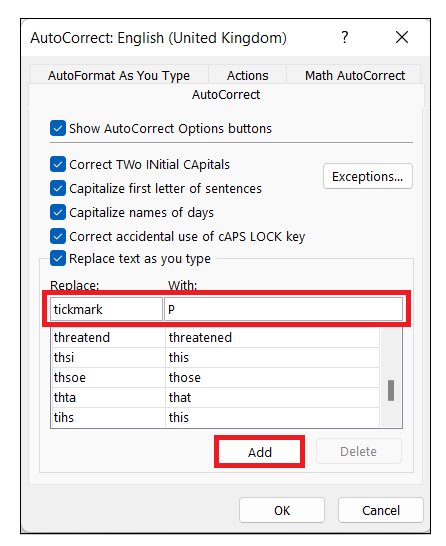
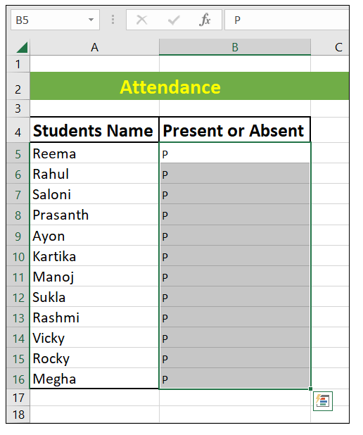
How to make a checkmark in Excel with AutoCorrect

If you use symbols quite often in your spreadsheets, there is an automatic method that you can use to add the tick and cross symbols. Perform the following steps to implement the automatic symbol method:

1. The first step is to insert a tick symbol (of any appearance that you like) in your cell using any method covered so far in this tutorial.
2. Copy the symbol from the formula bar by pressing the shortcut key Ctrl+C.

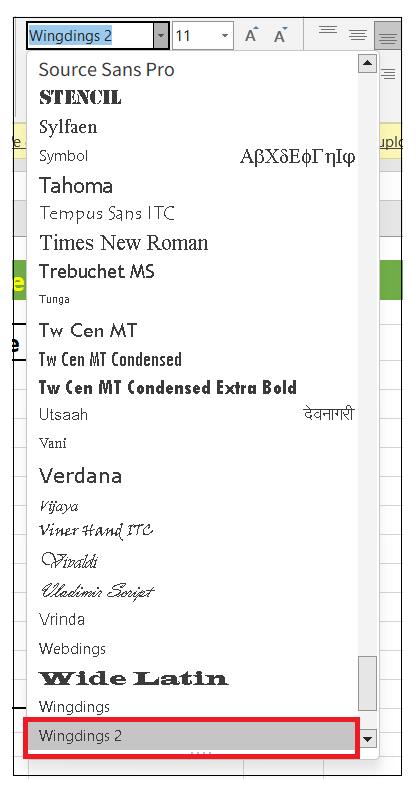
NOTE: In the formula bar, the appearance of the tick symbol may not look correct. Sometimes it seems different because you inserted a tick symbol in your worksheet using another Excel character code. From the font, Box selects a suitable font styling (in our case, we have chosen Wingdings 2), as later, the same will be copied to all other cells.

1. to the File menu. From the resulting window choose Options > Proofing > AutoCorrect Options?
   
2. The AutoCorrect dialog window will appear, apply the following rules:
   • Look for the Replace box in the dialog window, enter the text that you want to link the tick symbol with, for instance in your case we have associated it with the work "tickmark".
   • In the With Box, paste the symbol using CTRL + V that you have copied from the formula bar.
   • Once done, click on the Add button.
   • Click on OK and close the Options window.
   
   
3. Now, type the work tickmark in your Excel worksheet and press enter. You will have the following symbols in your worksheet.
   
4. As shown in the above screenshot, whenever you enter the word tickmark, it will autocorrect to the symbol P (that you have copied from the formula bar). To convert it back to the tick symbol, all you need to do is select the cell and select the appropriate font from the box. For instance, in this example, we will choose Wingdings 2.
   
5. The symbols will turn into tickmark as soon as you change its font. Refer to the following image.
   

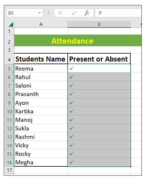
This method is one of the easiest, as you must configure and integrate the autocorrect options only once. After that, it will take the symbol automatically every you type the associated word in your Excel worksheet.

Insert tick symbol as an image

If you are not satisfied with the appearance of tick symbols applied in the above five methods and want to add some exquisite check symbol to your worksheet, you can also take the images from external resource (google or some other websites), download and copy the image and finally paste it to the selected cell.

For instance, here we have the below given tick and cross symbol, we have

1. Copy the image by using Ctrl + C shortcut key
2. Open your worksheet, select the cell where you want to paste the image. Now, press Ctrl + V to paste the image at the selected image.
3. The last step is to right-click on the tick mark, and click on the "Save image as?" option to save the image on your system.

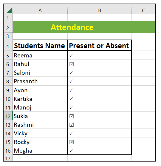
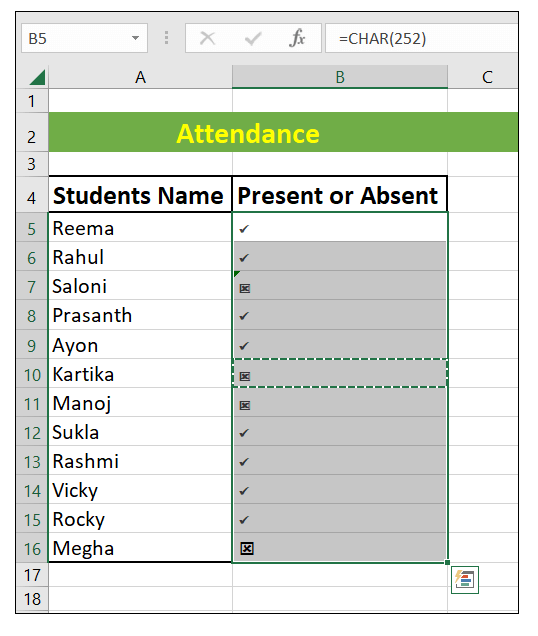
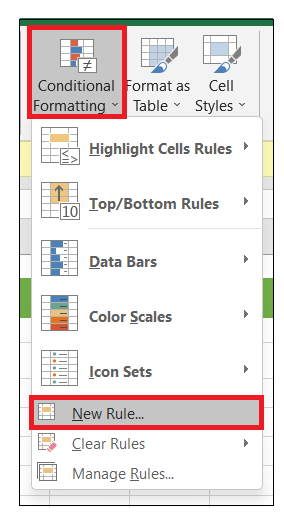
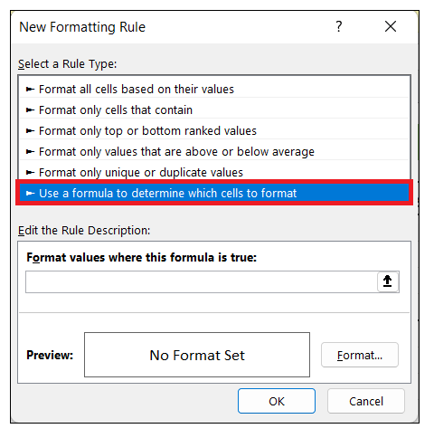
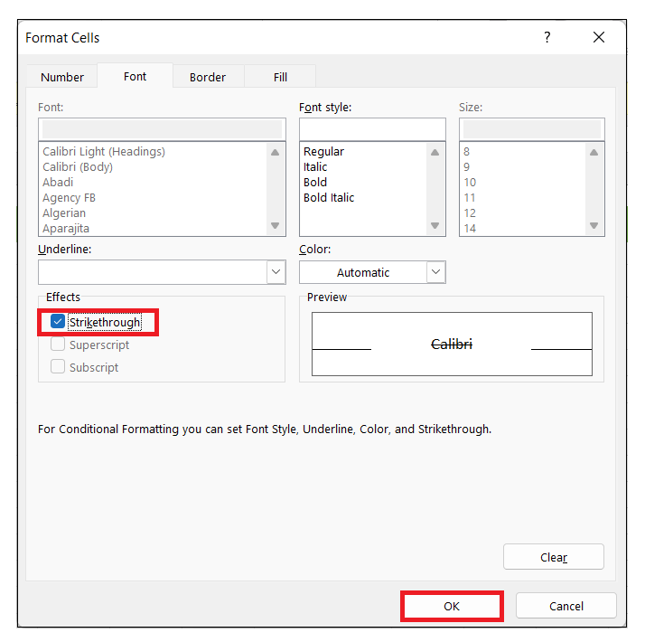
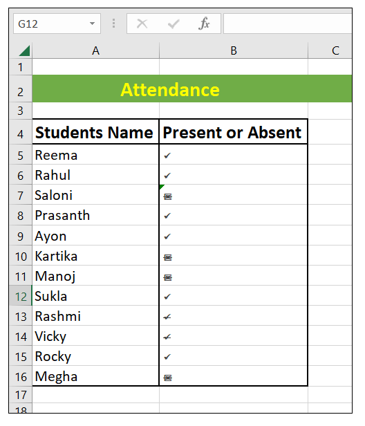
Conditional formatting on the basis of tick & cross symbol

Now that we have already covered different techniques to insert tick or cross symbols in Excel, let's move to its advanced version of applying some formatting.

Conditional formatting in an Excel tool helps the users to highlight particular values or make specific cells easy to recognise. If your cells contain only the tick and cross symbol, you can easily apply a conditional formatting rule in any format.

You can easily apply conditional formatting to the tick or cross marks if your cells do not contain any other data apart from these symbols. The advantage of this technique is that you need not re-format your cells manually when you delete the formatted symbol.

To create a conditional formatting rule for tick and cross symbol in Excel spreadsheet, follow the below-given steps:

1. Select the tick symbols cells that you would like to format. In our case, we have selected cell range B5: B16.
   
2. From the Home tab, choose the Conditional Formatting > New Rule?
   
3. The following New Formatting Rule dialog box will appear. From 'Select a rule type' menu select the 'Use a formula to determine which cells to format' option.
   
4. In the Format values where this formula is true box, enter below given CHAR formula.

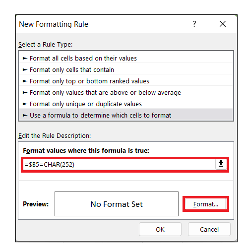
Note: To use the below formula, make sure you have applied the Char formula to create the tick symbols. Cell B5 represents the starting cell of your range.

Where B% represents the topmost cells containing the tick symbol, and 253 indicates the character code of the cross symbol that you have inserted in your worksheet.

1. Click on the Format option.
   
2. From the resulting formatting window, choose the required formatting style. In our case we have selected the strikethrough and click on OK button.
   
3. The result will look something similar to this:
   

You can try different conditional formatting and format the symbols per your requirement. All you need to know is the other character codes of the symbols. Go and give it a try now!

Points to Remember- Tick and Cross Symbol

We have almost covered all the topics related to Tick and Cross Symbol. But before giving closure to this tutorial, let's cover some essential points that will help you to master the topic completely.

1. Once you insert any symbol into a cell, it behaves like any other text. It means you can easily select, format or highlight the symbol as per your requirement. For instance, you can change its font size and colour or make it bold or italics.
2. You can also apply conditional formatting based on its colour or symbol type (using their character code). For instance, you can handle the tick symbol with a specific 252-character code, and it will apply the formatting specifically to the cells that contain the check symbol ignoring the other cells.
3. If you use Excel tick checkboxes instead of the tick symbols, you can even count the number of checked mark symbols, and finally can count the occurrence of TRUE values in the selected cells.

Hint - You can use the CHAR function to identify the cells containing a check symbol, and later on apply the COUNTIF function to count the cells. Check the formula below:

=COUNTIF(A2:A10,CHAR(252))

Where A2:A10 indicates the cell range for which you want to calculate the occurrence of check marks, and 252 represents the character code of the check symbol.