Percentage formula in Excel

What is Percentage?

A percentage is a number denoted in terms of the fraction of 100. The symbol of percentage is '%' and is displayed after a number. For example, 10 percent or 10% is written as 10/100. The percentage has no units.

The percentage has made the calculations even easier. It is sometimes difficult to represent a part infraction, such as one-twelfth, two-third, etc. But, it is easy to represent the fraction in percentage. Hence, the percentage is used everywhere in our daily life.

For example,

The fraction value 2/5th in percentage is written as 2/5 x 100 = 40%.

Percentage Formulas

A formula is an equation that performs the calculations. The calculations by humans are not accurate and quick. The calculations in excel are similar to the calculator. The percentage formulas are discussed below:

Selling price is the price at which the product is sold, while cost price is the price at which the seller purchased the product. Profit percentage is the profit earned from the sale of a product.

Loss is incurred when the cost price is more than the selling price. It means that the seller sold the product at lesser prices compared to the price they purchased.

We can also use the profit % formula to find the loss percent. The difference is that it will come in negative.

Where,

A and B are the commodities whose difference percentage is to be calculated.

Average is calculated as the sum of all the commodities divided by the number of commodities. We can also call it as a mean.

Let's first discuss some common features of excel.

• Data Sorting
  We can easily sort the data in excel by just few clicks.
• Built-in formula
  Excel has various built-in formulas that are visible on the tool bar present at the top. We can also compute the formulas on the formula bar.
• Data filtering and different charts
  It also the ability of data filtering and different charts, such as pie charts, bar charts, etc.

Excel provides us various ways to use the percentage formula, such as difference between two values, total percentage, percentage decrease, percentage increase, etc., as discussed above. We will discuss all the related examples for a better understanding.

So on moving forward, let us now first consider the steps which can be used to open an Excel file on the computer if someone needs to learn how to achieve this respectively.

Steps for opening an Excel file

Step 1: First of all, you are required to open the Excel file on your personal computer or desktop, then right-click on the home page -> select New -> and Click on Microsoft Office Excel Worksheet, as depicted below respectively: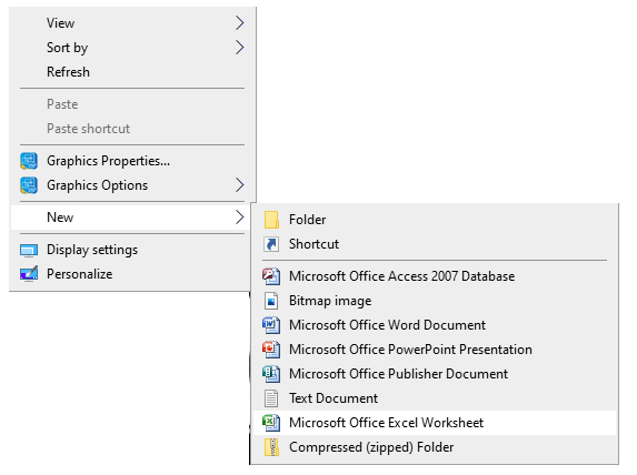

Step 2: Now, after that, you all need to specify the proper name for the file and then click on the newly created icon of Microsoft Excel on the home page.

Step 3: Microsoft Excel is ready for use after performing all the above steps.

Percentage formula

Excel has a built-in percentage symbol which is efficiently present on the toolbar. It is generally resent at the center of the toolbar, as depicted below:

To convert a decimal value into a percentage, specify the decimal value in an Excel block -> and click on the block, -> then click on the percentage symbol (%) on the toolbar. The corresponding decimal value will be getting converted into a percentage value.
Or

One can easily click on the decimal value block and press Ctrl + Shift + %. The corresponding decimal value will be getting converted into percentage values respectively.

Examples that are based on the percentage formula

Now let us discuss some examples of using percentage formulas in Microsoft Excel with the help of the various methods discussed below.

Example 1: Calculating the total percentage of five students in three subjects.

The data related to the 5 students in three subjects, English, Mathematics, and Science, is as depicted below:

And the steps which can be used to calculate the percentage of these three students are as follows:

Step 1: First of all, you need to click on the first block of the percentage column, as depicted below: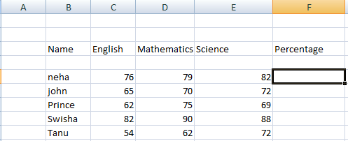

Step 2: After that, one must drag the mouse to the formula bar and type '= (click on the column number D + click on the column number E + click on the column number F)/300' respectively.

It will be then specified as '=(C: C+D: D+E: E)/300%.' Here, C: C, D: D, and E: E is the automatically specified name of the columns as well.

The percentage symbol will then automatically convert the data value into the percent.

We can also write the above formula as:

The formula of percentage is: '==(C: C+D: D+E: E)/300* 100'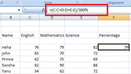
(Sum of numbers in all the subjects)/ Total marks x 100

Step 3: After that, you need to Press Enter button. The percentage value on the discount column's first block will appear respectively.

Step 4: Click again on the first block of the percentage column -> click on the bottom-right corner of that block, as depicted below: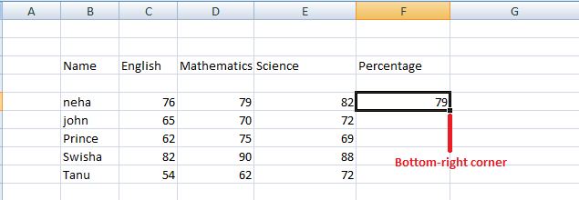

Step 5: Now, in this step, one needs to drag, that point to the fifth block of the same column (Percentage), as depicted below respectively: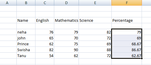

The percentage value will then be computed automatically. Similarly, we can calculate the percentage of many students in a class with a single click.

We can also make use of the direct method to calculate the percentage as well.

Example 2: To calculate the discount percentage in Microsoft Excel.

The cost price, as well as the selling price of the three products (sugar, wheat, and maize), is as depicted below: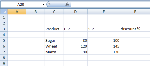

And to compute the discount percentage. We can easily insert the data under any column. The steps are as follows:

Step 1: Firstly click on the first block of the Discount % column, as depicted below: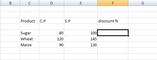

Step 2: After that, drag the mouse on the formula bar and type '= (1 - click on the column number E -click on the column number D)/ (again click on the column number D) * 100.' It will be specified as '(= (E: E-D: D)/D: D*100).' Here, E: E and D: D is the automatically specified name of the columns.

The formula for discount percentage is:
(Cost price - Selling price)/ Cost price x 100.

It will be getting appeared on the formula bar as in the image depicted below: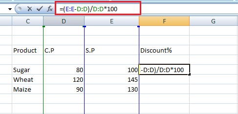

Step 3: Then press Enter button, and the percentage value on the first blockM of the discount column will also appear on the screen.

And the formula will also appear on the specified block, but as soon as we press Enter button, it will be replaced by the corresponding value respectively.

Step 4: Now, in this step, click again on the first block of the percentage column -> click on the bottom-right corner of that block,, as depicted below: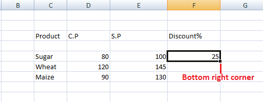

Step 5: After that, drag that point to the third block of the same column (Discount %), as depicted below: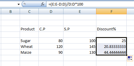

The percentage value will then be automatically computed.

Similarly, there are multiple numbers of the data rows. In that case, we can quickly scroll up to the desired data, which means we can compute the percentage of hundreds of data with just a single click. We are not required to calculate the percentage of the different products separately by using the calculator.

Example 3: To find the difference percentage between the two commodities.
Here in this, we will be finding out the percentage difference that lies between the two commodities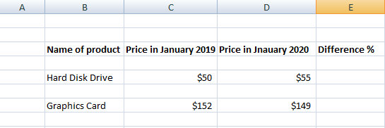, and the data is as depicted below:

And the steps that can be used to compute the percentage are as follows: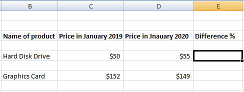
Step 1: First of all, one needs to click on the first block of the 'Difference %' column, as it was depicted below:

Step 2: After that, we must drag the mouse to the formula press and type '= (Click on the column D/Click on column C - 1) *100.' It will then appear on the formula bar as '= (D: D/C: C - 1) *100.' We can also write it as '= (Click on column D - Click on column C)/Click on column C x 100.'

And the formula for the discount percentage is as follows: (Price in 2020/price in 2019) - 1 ) x 100

Note: It should be noted that the percentage symbol in front of the difference value will not appear by default.

In case we want the percentage symbol to get appear in front of the difference% values, we need to follow the below steps as well:

Right-clicking on the difference% values -> select the Format cells option -> Click on the Percentage option on the left side of the window -> and click on the Ok button.

The percentage symbol will get appear on our screen as well. The percentage option selected here automatically converts the difference value into the percentage. '= (D: D/C: C - 1)'

So, we need not multiply the difference value by 100 to convert it into a percentage. The formula on the formula bar will appear as follows:

Step 3: Now, in this step, one needs to press the Enter button from the keyboard. The percentage value on the first block of the Difference% column will appear. The formula will also appear on the specified block, but as soon as we press Enter, it will be replaced by the corresponding value respectively.

Step 4: After that, click again on the first block of the percentage column -> click on the bottom-right corner of that block, as depicted below: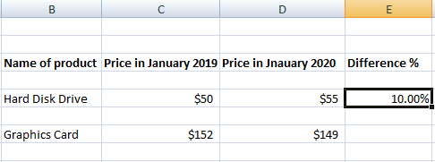

Step 5: Drag that particular point to the second block of the same column (Difference %), as depicted below: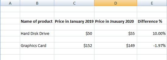

The second value of the difference percentage is negative (-1.97%), which means that the price of graphics cards has decreased compared to the previous year. Hence, Microsoft Excel is beneficial in quickly predicting the profit, loss, increase, or decrease of the price compared to the overall data.

Example 4: To find the profit and loss percentages of the seven products.
The data for the seven products 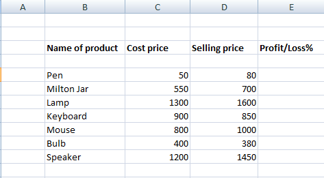are listed below respectively:

And the steps that can be used to compute the percentage are as follows:

Step 1: Firstly click on the first block of the 'Profit/Loss %' column, as depicted below: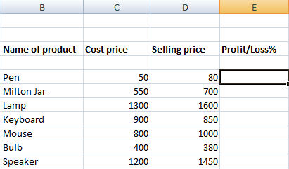

Step 2: Now, in this step, one needs to drag the mouse on the formula press and will then type'= (Click on the column D/Click on column C - 1) *100.' It will appear on the formula bar as '= (D:D/C: C - 1) *100.' We can also write it as '= (Click on column D - Click on column C)/Click on column C x 100.'

The formula for discount percentage is:

(Selling Price/Cost price) - 1) x 100

If the percentage value is positive, there is a profit, and if it is negative, the seller has incurred a loss.

The formula on the formula bar will appear as depicted below: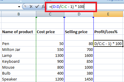

Step 3: After that, one must press the Enter button from the keyboard. The percentage value on the first block of the Profit/Loss% column will appear respectively.

The formula will also appear on the specified block, but the corresponding value will replace it as soon as we press Enter.

Step 4: Click again on the first block of the percentage column -> click on the bottom-right corner of that block, as depicted below: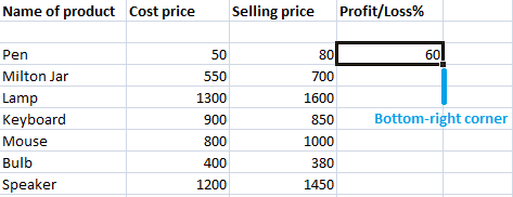

Step 5: Drag that point to the seventh block of the same column (Profit/Loss %), as depicted below: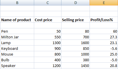

The above table shows the seven products' profit/loss percentages. But how can one conclude which product was sold at a profit and which at a loss? So, let's discuss it.

If the profit/loss percentage is positive, the product was sold at a profit, and if the percentage is negative, the product was sold at a loss. Thus, the keyboard and the bulb were sold at a 5.6 and 5 percent loss. Similarly, pens, jars, lamps, mice, and speakers were sold at a profit of 60, 27.3, 23.1, 25, and 20.8 percent, respectively.