| |

Excel VLOOKUP from Another SheetWhat is called Excel VLOOKUP?Coordinating or calculating the massive amount of data in the worksheet is a time-consuming and difficult process. To rectify this problem, the concept called VLOOKUP is discussed in this article. As the name suggests, VLOOKUP is called Vertical Lookup, which searches the data across the columns in the worksheet. It helps to compare and coordinate two data present in the worksheet, which saves the user's time. Working process of VLOOKUP Function in ExcelThe VLOOKUP function looks for the specified data vertically in the worksheet columns, and if the data is founded, it displays some information that is related to that data. Features of VLOOKUP Function
Syntax VLOOKUP (lookup_value, table_array, col_index_num, range_lookup) Lookup_value - The value which needs to be searched in the first column. Table_array - The table array is mentioned to retrieve the value from the table. col_index_num - It represents the column where the value needs to be retrieved. range_lookup- It has two options and is optional too. The first one is TRUE, as it denotes the approximate match. The TRUE value is present as a default option. The second one is FALSE, as it denotes the exact match. An example of the VLOOKUP function is as follows, Example 1: Display the selected data using VLOOKUP Function Step 1: Enter the data in the worksheet, namely A1:F6. 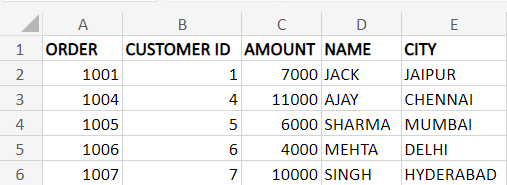
Step 2: Here, the name of the Order 1005 needs to be displayed. Select a new cell namely F1 and enter the formula as =VLOOKUP (1005, A2:E6, 4, FALSE) Step 3: Press Enter. The VLOOKUP function returns the name SHARMA. 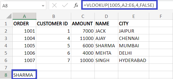
Here the lookup value is 1005, the table array is A2:E6, the Column index number is 4, and the range lookup FALSE indicates the exact match. From the above example, the VLOOKUP function is searched in a single worksheet. The concept of using the VLOOKUP function in the same Sheet for fetching the data is explained. How to work in two worksheets using the VLOOKUP function?Sometimes the user needs to compare the values with another worksheet or Workbook. To perform this action, the VLOOKUP function is used, which performs the task easily and reduces the manual working process of the user. The various examples of the VLOOKUP function are as follows, Example 1: Using the VLOOKUP function, display the required data in two different worksheets but the Same Workbook Step 1: Enter the data in the worksheet1 namely A1:D11 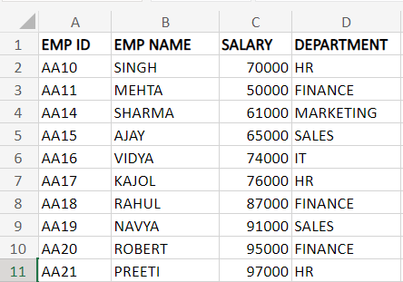
Step 2: Copy the Employee ID and Salary in another worksheet in the same Workbook. 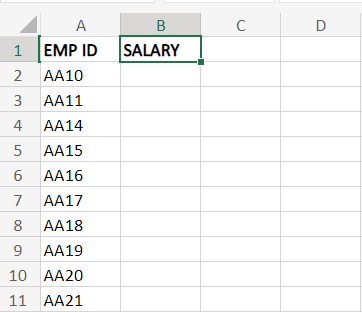
Step 3: The sheet1 and 2 are named based on the user's choice. Here sheet 1 is named a Data Sheet, and sheet 2 is named a Result sheet. Step 4: In the result sheet, enter the formula in the cell B2 as =VLOOKUP (A2,' DATA SHEET'! $A$2:$D$11, 3, 0). While typing the formula, the user need not manually type the worksheet's name. While clicking the name of the first worksheet (DATA SHEET), it automatically fills the name in the formula. 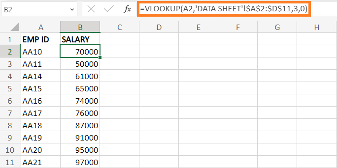
Step 5: The SalarySalary will be displayed in cell B2. Drag the formula towards the remaining data, B11, to get the result. In the formula, A2 is called the lookup value, DATA SHEET is the name of Sheet 1, A2:D11 is the table range, 3 is the column index number, and 0 is the row number. Example 2: Using the VLOOKUP function to display the required data in two different worksheets but the Same Workbook In example 1, the data fetched from the different worksheets in the same Workbook is explained. Here in this example, the concept of fetching the data in different Workbooks is explained here. In this example, the data is fetched from Data Workbook to Result in Workbook. Step 1: Enter the data in the worksheet, namely A1:D11. The first workbook name is named Data Workbook. Step 2: Enter the Employee Id and Salary in another worksheet, Result Workbook. Step 3: In the Result Workbook, select cell B1 and enter the formula as =VLOOKUP (A2. Then go to the Data Workbook and select the range to display in the Result Workbook. It automatically updates the formula. Here the path of the Data Book is updated in the Result Workbook. Step 4: The result will be displayed in the cell B1 of the Result Workbook. To get the result for the remaining data, drag the formula toward cell B11. 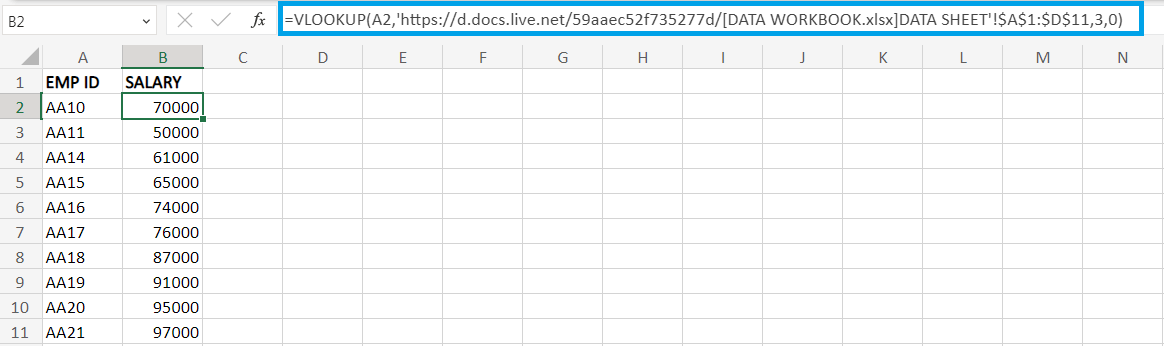
In the worksheet, the path of the Data Worksheet is highlighted, which is used to retrieve the necessary data from the Data Worksheet. Note: The table array should be locked if the formula is applied to a different Workbook because it automatically makes it an absolute reference.The table array should be locked if the data is fetched from the same worksheet or a different worksheet of the same Workbook. It is suggested to remove the VLOOKUP function if the data fetching process is done in another worksheet. The data present in the Workbook is lost if the Workbook is deleted. Example 3: Retrieve the specified data using the VLOOKUP function in the worksheets of the same Workbook. Step 1: Enter the data in the worksheet, namely Sheet 1 from A1:B11 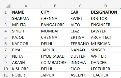
Step 2: Enter the 'Name' column in the next Sheet, Sheet 2. Step 3: To find the car name of all persons in Sheet 2, select cell B2 in Sheet and enter the formula =VLOOKUP (A2,' SHEET 1'! $A$2:$D$11, 3, 0). The data will automatically display in cell B2. To get the result for the remaining data, drag the formula toward cell B11. 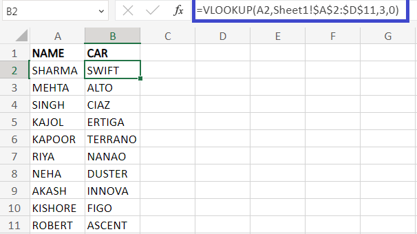
The person's car name is filled in the worksheet using the VLOOKUP function. Similarly, this method is followed to retrieve the specified data for the other example. The formula A2 is called the lookup value, SHEET 1 is the name of the Sheet, A2:D11 is called the table range, 3 is the column index number, and 0 is the row number. Example 3.1: Retrieve the specified data using the VLOOKUP function in the worksheets of the same Workbook. In example 3, the name of the person's car is retrieved from Sheet 1. In this example 3.1, the person's Designation is retrieved in Sheet with a little modification in the formula. In Sheet 2, in cell B1 enter the formula as =VLOOKUP (A2,' SHEET 1'! $A$2:$D$11, 4, 0) Here in the formula, A2 is called the lookup value, SHEET 1 is the name of the Sheet, A2:D11 is called the table range, 4 is the column index number, and 0 is the row number. The column index number is modified here as the Designation is present in the fourth column. The VLOOKUP function retrieves the designation column from Sheet 1 and displays it in Sheet 2. 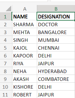
From the worksheet, Designation is displayed in the worksheet. Example 3.2: Retrieve the specified data using the VLOOKUP function in the worksheets of the same Workbook. In example 3.1, the person's Designation is retrieved from Sheet 1. In this example 3. 2, the person's City is retrieved in Sheet with a little modification in the formula. In Sheet 2, in cell B1 enter the formula as =VLOOKUP (A2,' SHEET 1'! $A$2:$D$11, 2, 0) Here in the formula, A2 is called the lookup value, SHEET 1 is the name of the Sheet, A2:D11 is called the table range, 2 is the column index number, and 0 is the row number. The column index number is modified here as the City is present in the Second column. 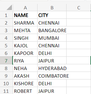
The VLOOKUP function retrieves the CAR column from Sheet 1 and displays it in Sheet 2. Example 3.3: Retrieve the specified data using the VLOOKUP function in the worksheets of the same Workbook. In example 3.2, the City of the person is retrieved from Sheet 1. In this example 3. 3, the person's SalarySalary is retrieved in Sheet with a little modification in the formula. In Sheet 2, in cell B1 enter the formula as =VLOOKUP (A2,' SHEET 1'! $A$2:$D$11, 5, 0) Here in the formula, A2 is called the lookup value, SHEET 1 is the name of the Sheet, A2:D11 is called the table range, 5 is the column index number, and 0 is the row number. The column index number is modified here as the SALARY is present in the FIFTH column. 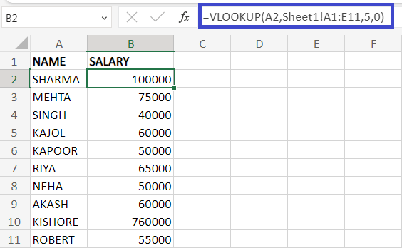
From the worksheet, the salary column is retrieved in Sheet 1 and displayed in Sheet 2. SummaryThe tutorial explains the methods to retrieve the data from the same worksheet or worksheets in the same Workbook or Workbooks. |
 For Videos Join Our Youtube Channel: Join Now
Feedback
- Send your Feedback to [email protected]
Help Others, Please Share


