OR Function in ExcelWhat is OR Function in Excel?The OR function is a built-in function in Excel that belongs to the Logical Function category. The OR function can be used as a worksheet function (WS). Like a worksheet function; the OR function can be entered as a part of a formula in a worksheet's cell. The OR function returns TRUE if any of the conditions are TRUE, and it returns FALSE if all conditions are false. Up to 255 parameters can be passed to the OR function, each of which is a logical test. There is only one argument necessary. However, if we are using OR function, we probably have at least two. SyntaxThe syntax of the OR function is: ParametersThe following are the parameters of the OR function:
condition1: -A condition to test that can either be TRUE or FALSE. condition2, …condition_n:- Optional. Test conditions that can be either TRUE or FALSE. There can be up to 30 conditions. Returns
When to Use OR Function?We used OR function when we need to verify many conditions in a defined cell. Things to Remember About OR Function in ExcelThe following are the things which we have to remember about OR function in Excel:
How to Use the Excel OR FunctionLet us discuss how to use Excel OR function with the help of the examples: Example 1: Here's an example of how to utilize the OR function practically. The Sales Department would like to reward all employees of the South team for outstanding overall performance, as well as anyone from any other team who has made more than 32 sales. An employee would be eligible for the incentive if any of these two conditions were met. 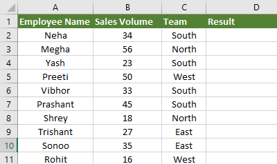
If we want to know the rows that satisfy one or both criteria, two statements are required. The first statement asserts that the value in cell B2 is greater than 32, whereas the second asserts that the value in cell C2 is the word "South." The OR formula would be as follows: 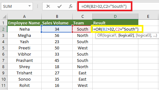
The result TRUE is shown if both statements are true or if at least one of the statements is true. The result FALSE is displayed if neither statement is true. 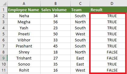
Use with the Filter FeatureWith the Filter feature, we can also use the OR function. It works well with this feature because it is straightforward to show only those rows that meet at least one of the mentioned criteria and hide those that do not. 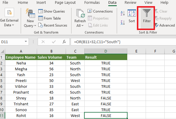
From the Data tab on the ribbon, we have to click on the Filter icon and use the filters arrows at the top of the dataset to select the rows containing a TRUE value in column D. Then, we have to click OK in order to apply the filter, as we can see in the below screenshot: 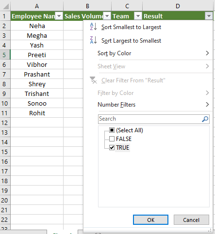
Rows that do not meet either of the mentioned criteria are filtered out of the display, as indicated by the blue row numbers. 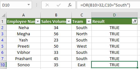
Example 2: OR Function with the IF Function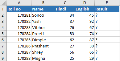
The OR function can also be used with the IF function. In this example, we have a data set that contains students' marks of two subjects: Hindi and English. If Hindi marks are above 45 and English marks are above 40, the student is considered a pass. To find out the pass students, we have to apply the following formula: 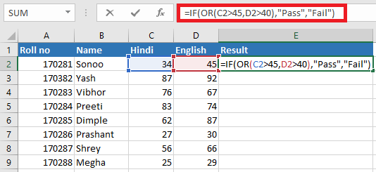
After applying the formula, we get the below output: 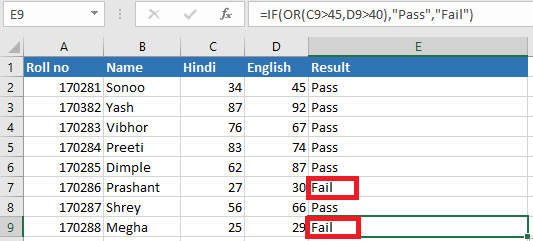
As we can see in the above screenshot, Roll no. 170286 and 170288 has less number in both subjects Hindi as well as English as per the argument or condition requires; hence they are considered FAIL. Roll no. 170286 has 27 marks in Hindi and 30 marks in English and required is 45 and 40, respectively, hence the result is FAIL. Same with Roll no. 170288. Example 3. Use IF/OR Combination with a Mathematical Calculation.In this example, we will use the IF/OR function with mathematical calculation for the value_if_true. The spreadsheet below shows the number of times a company's website has been visited in the last 30 days and the previous 30 days. 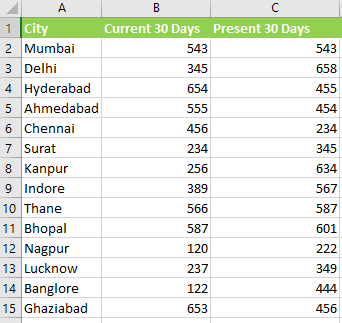
If either column B or column C contains a value greater than 600, it is considered a high-traffic location. We need to determine which cities have high traffic locations and the average number of visits for the two months included in the report. If a city is not considered a city with high traffic, no average should be calculated. The IF and OR function would be nested for Argument 1 in the same way as in the previous example. The AVERAGE FUNCTION would be used as the second argument: The third argument can be omitted to return a FALSE value, indicating those cells that did not meet any of the given criteria. The full formula would read: 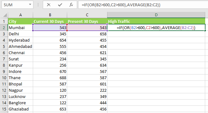
When we copied the above formula to all the relevant cells in column D, the worksheet's outcome is: 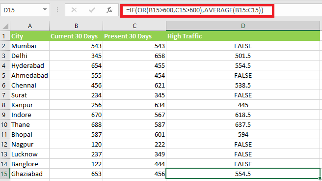
Use with Sorting The sorting feature may now be used to create a list of cities sorted by traffic volume from high to low or low to high. 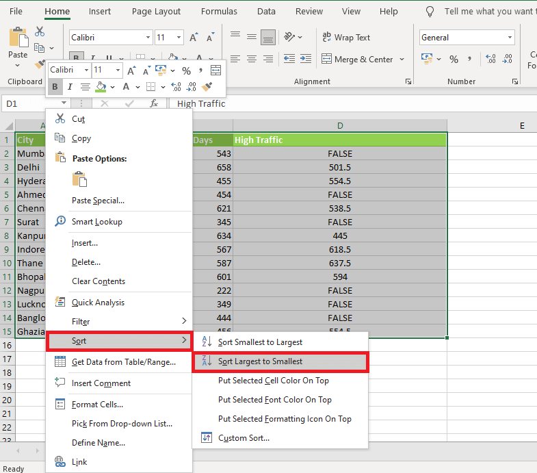
We will get the below result after applied the feature of sorting: 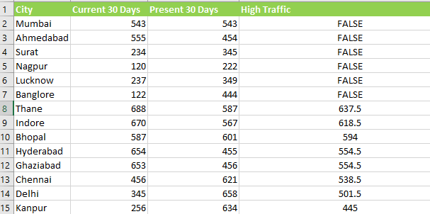
SummaryThe Excel OR function can be used to execute several tests within a single function to find cells that fulfill various criteria. Because of the OR function's simplicity, the logic is simple to understand and can be used for almost any sort of dataset. It is highly useful and adaptable when used in conjunction with other Microsoft Excel functions and features.
Next TopicSolver in Excel
|
 For Videos Join Our Youtube Channel: Join Now
Feedback
- Send your Feedback to [email protected]
Help Others, Please Share


