How to format Excel Sheet

What is called Formatting the Excel sheet?

Excel spreadsheet is used for multiple purposes for various requirements such as business, finance, budget planning, student's mark sheet, attendance, etc. After finishing the organizing data in a spreadsheet, the worksheet must be formatted. Formatting helps the worksheet look more attractive and professional way. It helps the user to understand the data quickly and effectively. Based on requirements, the spreadsheet is formatted. Overall, formatting the spreadsheet gives the data clarity, consistency, and efficiency.

How to format the Excel Spreadsheet?

There are several techniques to format the Excel Spreadsheet. Some of the methods are as follows,

1. Coloring the Text

Coloring the text helps to differentiate the data present in Excel. For data like finance, budget planning, company profit, etc., coloring the text with different colors helps quickly understand the data.

For example, in student's attendance sheets, to identify the data quickly the colors are used such as,

• Blue color for students' Names.
• Brown color for Present Students
• Orange for Absent Students
• Green for students who scored above 75%
• Red for students who scored below75%

To color the text in Excel, the steps to be followed are as follows,

1. Select the cell containing the specified text.
2. Select the drop-down menu, which is present next to the Font color icon.
3. There displays a palette that contains various colors. In that, choose the required color to color the text.

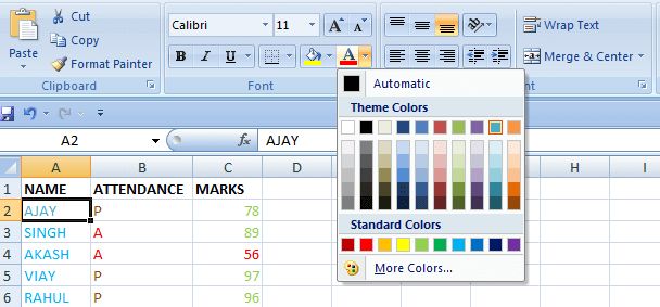
2. Bold and Italic Format

The Bold and Italic option highlights the specific text clearly and differentiates it from other data. Bold is used for emphasis, and Italic is used to indicate the specific data.

For example, if the spreadsheet contains the data regarding percentage and total, the percentage is indicated in italics, and the total is indicated in bold.

To make the text bold or italic, the steps to be followed are,

• Select the cell which needs to be changed into bold or italic
• Choose the required option in the Home tab, such as Bold or Italic. The selected text will change into bold or italics.

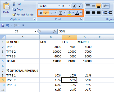
Here the selected texts are changed to bold and italic format.

3. Conditional Formatting

As the name suggests, the conditional formatting option highlights the cells based on conditions. The conditional formatting option is used if a large data set contains several values that need to highlight the specified cell based on conditions.

To use Conditional Formatting in Excel, the steps to be followed are:

For example, to highlight the duplicate values in the data, the method to be followed is:

1. Enter the data in the cell range, namely A1:A10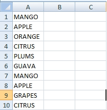

2. Select the cell range from the data A1:A10, and choose the Conditional option Formatting in the Style tab from the Home tab.

3. There display several options in that choose the option Highlight Cell Rules. In Highlight Cell Rules, select the option called Duplicate Values.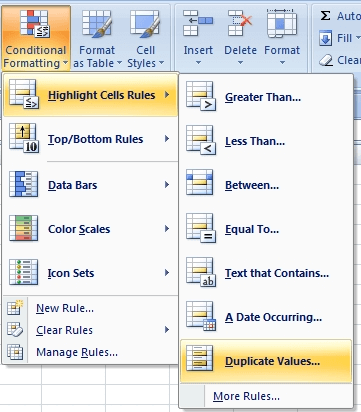

4. The Duplicate values dialog box will appear. In a drop-down list, choose either unique or duplicate values. Here the duplicate option value is selected. Choose the specific color which highlights the duplicate values.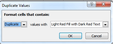

5. The Duplicate Values are highlighted with Light Red and filled with Dark Red Text.

4. Using the Fill Handle option

The Fill Handle option is used to fill the series of data in the specified cells following the same pattern in the data. The Fill Handle consists of four options such as,

• Copy Cells
• Fill Series
• Fill Formatting Only
• Fill Without Formatting

The Fill Handle option is used to fill the cells across the right, towards the left, and down from the selected cells.

To use the fill handle, the steps to be followed are:

Enter the data in the required worksheet.

Choose the specified data, and drag the fill handle toward the specified direction.

The Auto fill option will display; in that, choose the required option.

The Copy cell option copies the current cell value to the selected cells.

The Fill series option fills the selected cell with numbers from the existing cell.

The Fill Formatting Only option fills the specified cells with the formatting option only, not the values.

The Fill Without Formatting option fills the data with values and not the formatting option.

5. Format Painter Option

The Format Painter is an option in Excel used to copy the formatting option from the specified cell or range to another cell or range. It saves a lot of time for the user.

To use the Format Painter Option, the steps to be followed are:

1. Enter the data in the worksheet, namely A1:A5. In the data from cell A1:A5, the cells are formatted with selective patterns.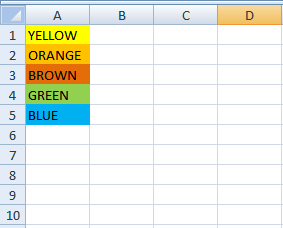

2. To follow the same pattern for the cell range B1:B5, select the cell range A1:A5 and click the Format Painter option in the Clipboard Section of the Home tab.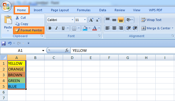

3. Now, Click cell B1 where the formatting pattern in cell range A1:A5 is copied to cell range B1:B5.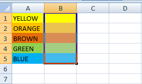

6. Formatting the Data As Table

Formatting the Data As a Table is one of the various features in Excel. When adding a new value, the table automatically expands by formatting the data as a table. Features like filter icons and headers are added. It makes data organized and easier to understand. When the formula is edited or added, it automatically copies down to the column and when a new row is added.

To format the data as a table, the steps to be followed are,

1. Enter the data in the worksheet, namely A1:D5. Select the necessary data in the worksheet, which needs to be formatted as a table. Here the range A1:D5 is selected.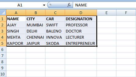

2. Now choose the "Format as Table" option, which is present in the Style Group of the Home tab.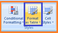

3. There display several patterns. Choose the required pattern to format the data as a table.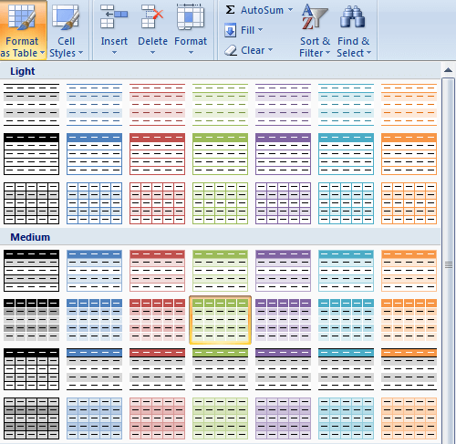

4. After choosing the required pattern, a "Format as table" dialog box is displayed. If there is no blank cell, It displays the selected table range. Else, the data needs to be entered manually in the blank cell. Select the option "My table has a header." Click OK.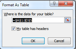

5. Now the data is formatted as a table.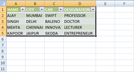

7. Formatting Numbers

The formatting Number option in Excel is used to format the numbers based on the data requirement, like Dollars, Percentages, and decimals in Finance, Budget Planning, etc.

To format the numbers in Excel, the steps to be followed are:

1. Enter the data in the required worksheet, namely A1:B11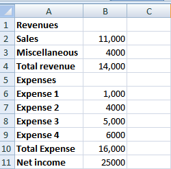

2. To format the value in cell B2, select cell B2, and choose the Accounting Number Icon present in the Number group in the Home tab.

3. A dollar sign is inserted in front of the value present in cell B2.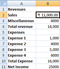

4. To add the decimal point in cell B6, select the cell and click the Increase Decimal option in the Number group in the Home tab.

5. The specified decimal point is added to the value present in cell B6.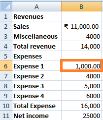

6. Select the required cell to decrease the decimal point; here, the cell selected is B6. Click the Decrease Decimal option in the Number group in the Home tab.

7. The specified decimal point is decreased to the value present in cell B6.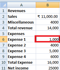

The Format Painter option is also used to format large datasets of numbers.

8. The comma sign in the Number group in the Home tab is used to insert a comma to the selected value, and automatically, two decimal points are added. To remove the decimal point, select the Decrease Decimal Point option.

Another method to format the number is using the Format option. The steps to be followed are:

1. Select the cells containing values that need to be formatted.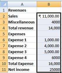

2. Click the Format Option in the Cells Group in the Home tab. Select the Format Cells option.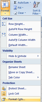

3. The Format Cells dialog box will appear. In that, choose the Number option. Choose the Accounting option in the Category List.

4. Enter the required number of the decimal point in the Decimal places which need to be added to the value. Here two decimal point is added.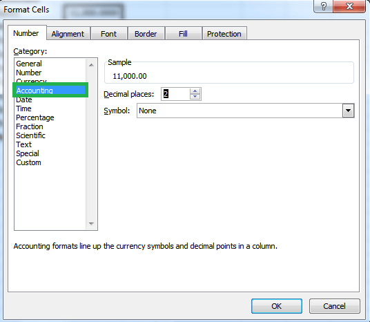

5. Now the required decimal point is added to the selected cells.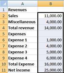

9. Formatting Percentage

Percentages are used in Excel for calculations regarding profit, rate of interest, budget, tax and revenue, proportions, etc.

To format the percentage, the steps to be followed are:

1. Enter the data in the required worksheet.

2. Select the necessary cell containing the value that needs to be formatted to percentage. Here cells B7 to B9 are selected.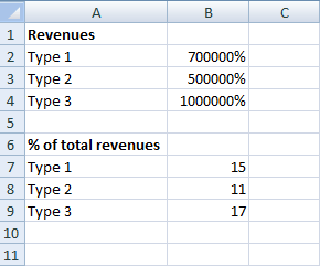

3. Choose the Percentage symbol present in the Number group in the Home tab.

4. Now, the selected cells are formatted with percentage values.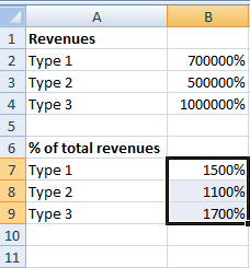

5. If two decimal points are present in the worksheet, they can be removed using the Decrease Decimal option present in the Number group of the Home tab.

10. Formatting Dates

Formatting the Dates based on the desired pattern helps to organize the data and perform the calculations easily and quickly. It is used in various fields such as Finance, Accounts, Economics, etc.

The steps to Format the Date are as follows:

1. Select the number format in the Number group in the Home tab. There display several options, called "Short Date" and "Long Date."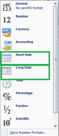

2. Choose the option called "More Number Format." The Format cell dialog box will appear. In the Number tab, choose the option called "Date."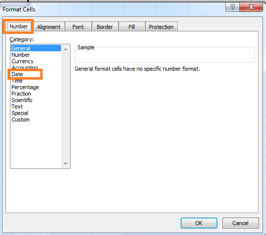

3. The Date option displays various types of date formats. In that, choose the desired format applied to the selected data.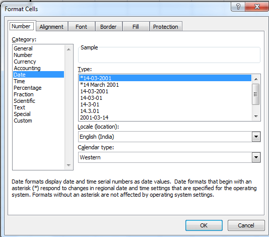

Summary

The various steps to format the Excel spreadsheet are described in this tutorial. Various formatting options are present in Excel; based on the data required, the Excel sheet is formatted, making the data attractive and organized.