Excel RAND() function

RAND() is a function that is categorized into Math & Trigonometry category in Excel. It returns a random number between 0 and 1. This random number is greater than or equal to 0 (>=0) and less than 1 (<1).

Excel RAND() function does not take any argument and the result of this formula is volatile. You are now wondering that how this formula works and why it is used.

In this chapter, you will learn the usage of RAND() function, properties, examples, and other things to guide each step in detail. Additionally, we will also brief why use this function.

Syntax

It is a simple function without any argument.

What does it returns?

As it calculates a random number between 0 and 1, it returns it back to the user.

Purpose of RAND()

The RAND() function generates a random number between 0 and 1. Each time formula recalculates when an Excel worksheet opens and closes.

Specify the range by own

Additionally, you can also set your own range to get a random number to be chosen from between it. For example,

Here, b is the largest number and a is the smallest number of the defined range.

Note: This function will never return the random number greater than the largest number.

Example,

The above formula will generate a random number between the range of 10 to 24.9999.

We have a list of examples in a table in which you can analyze that how different this function works and what it returns.

However, you can also use RANDBETWEEN() formula for this purpose. Excel enables you to customize the RAND() function according to your need and do the same thing as RANDBETWEEN.

Why this function is needed?

The RAND() function generates a random sequence of numbers. Sometimes, an Excel user requires to assign random numbers or tasks. You can do it by using this function.

It will help the Excel users to assign a random number or task to a group of people by assigning them a random number.

We are going to discuss the following example in this chapter:

• Example 1: Simple RAND() implementation
• Example 2: Customize result
• Example 3: Generate integer random number
• Example 4: Random assignment of task

How to use RAND() function?

To understand where and how to use RAND() function, you have to learn it with example by applying it to Excel data. We will give you two-three examples of this function that will help you to learn this function.

Now, we will implement the RAND() function to Excel data. For this, we have taken this numeric set of data.

Example 1: Simple RAND() implementation

Step 1: Firstly, we have not specified anything. We will simply use RAND() function on this worksheet. So, write

=RAND()

Anywhere in your Excel sheet.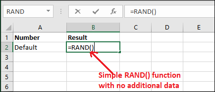

Step 2: Get the result by hitting Enter key. You can see a random number is returned by this function between the range of 0 to 1.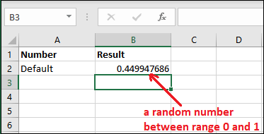

Step 3: This random number will change whenever you will try to add, delete, or perform any other operation on the same Excel sheet.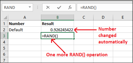

You can see that while performing one more RAND() operation, the previous result has changed.

Step 4: Each time you use this function, it will return a different random number. This number will not be the same each time. Look at for new random number -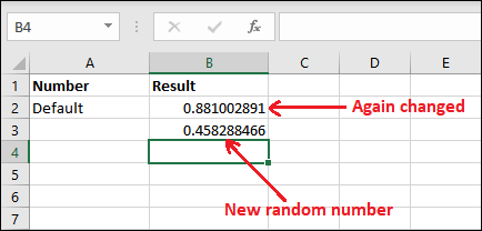

You can see that the previous result has changed one more time.

Note: These random numbers will change each time with worksheet modification and even if the worksheet will open or close.

Example 2: Customized result

Excel allows the users to customize the result of between 0 and 1. Although you cannot provide parameters to RAND() function but you can decide the range of the random number to be generated.

For example, generate a random number between 0 and 100 because the default start range is 0. For this, you have to define the range with the RAND() function by multiplying with it.

Let's see how it would be done with RAND() function:

Step to customize RAND() function result

Step 1: In this Excel worksheet, we have defined the range in column A and in column B we apply RAND() formula for a specific range and get the result.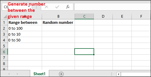

Step 2: Write the RAND() formula with a specific range like this:

=RAND()*100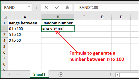

Step 3: Now, get the result for the above formula and see what it returned.

You will see that it has returned a random number 82.03015662 that is below 100 and above 0.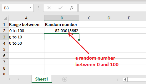

"You don't need to put too much effort, you just multiple the RAND() function with the range within which you want get the random number."

Step 4: Now, let's get a number between 0 to 10. Use the following formula -

=RAND()*10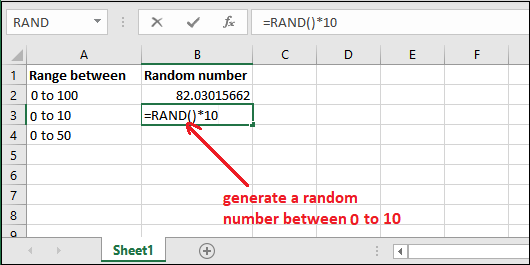

Step 5: Now, See the result for above formula calculation this will return the result between 1 to 10.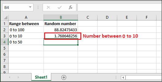

Similarly, you can generate the random number for any given range by specifying the range in multiple number.

Generate a number between two numbers

Besides this, you can define the start range along with the end range as well. We have another formula for it. Use the formula =RAND()*(endRange-startRange)+startRange.

Step 6: Here, we have specified the start range 20 and end range 50. Write the formula in C2 cell -

=RAND()*(B2-A2)+A2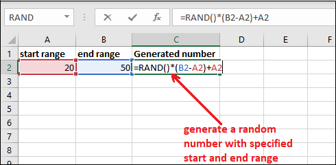

Step 7: Hit the Enter key and get the generated number of between 20 and 50.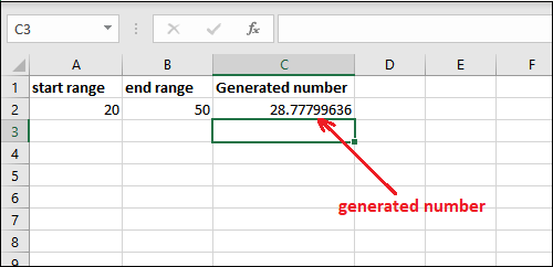

Using this formula, the generated random number will never be greater than end range and smaller than start range.

Example 3: Generate integer random number

In all the above examples, you have noticed that the RAND() function is generating a number with a decimal point. If you want this number is an Integer, you have to use INT() function.

Remember you have to define the range more than 1. Otherwise, the default range for RAND() function is 0 to 1. See an example for it below:

Step 1: We have used the RAND() function with INT() to get the generated number as an integer.

=INT(RAND()*100)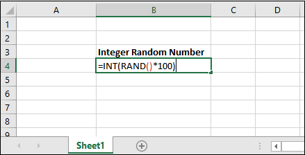

Step 2: See that it has returned as integer value less than 100.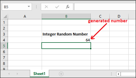

Example 4: Random assignment of task

Let's take a scenario and see an example for random assignment of a task to a group of people by using Excel RAND() function. For example,

We have a group of people data stored in an Excel sheet whose we want to assign the task randomly. Use the RAND() function of Excel. See the initial data we have -

Step 1: Initially, we have a list of five people in column A (cell A2 to cell A6).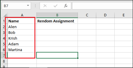

Step 2: Select the all given data (A2-A6) and take the mouse control over A6 cell bottom right corner where you will see an + sign. Drag this + sign to row 20.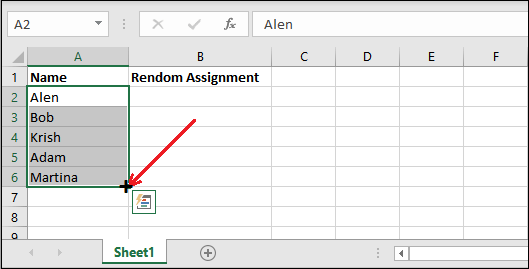

Step 3: You will see that the data is regenerated for till row 20.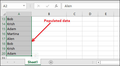

Step 4: Leave column B blank for now and type two sequential numbers in C2 and C3 cells as showing here.

Select those numbers and drag to row 20 as in steps 2 and 3.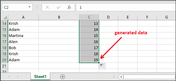

Step 5: Now, type the Excel RAND() formula firstly in D2 cell to generate a random number.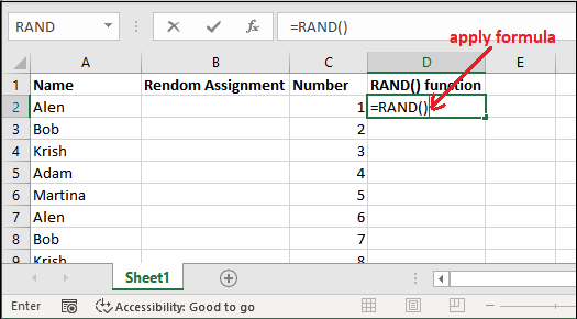

Step 6: Select the D2 cell and drag the mouse till row 20 as in previously performed steps.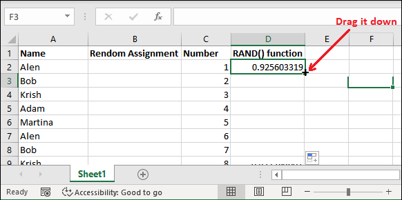

Step 7: It will automatically generate the random number for all the rows till 20. See the given screenshot.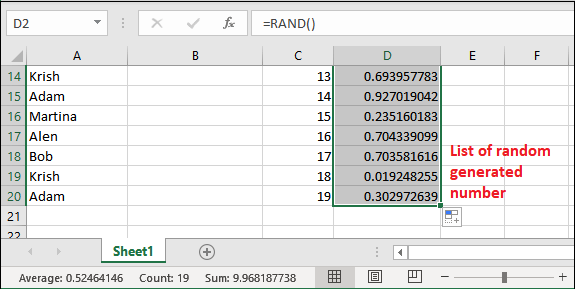

Note: These generated random numbers are unordered.

Step 8: Right-click any of the random numbers of column D and click on Sort then select Sort Smallest to Largest.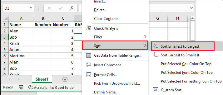

Step 9: The generated random numbers will be sorted from smallest to Largest. You will also see that the position of the column A and column C elements has also been changed.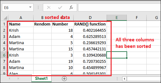

Step 10: Finally, delete column D and column B (the blank column).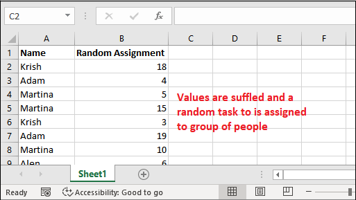

Additional information about RAND()

RAND() function comes under Math & Trigonometry function category. You can do more things with this function while applying it on your Excel sheet -

1. Each time RAND() function calculates a new value whenever the Excel worksheet is opened or closed. If you want to prevent the recalculation and stop the regeneration of this random number, convert the number value to text by using Paste Special > Values of Excel.
2. If you wish to generate a set of random numbers for multiple cells, selects the cells, enter =RAND() formula and then press the Ctrl+Enter
3. This function generates a new random number each time the worksheet is calculated. If you want that this result will not change, enter the formula and press F9.
4. If you wish to generate a random of your defined rather than default 0 and 1. You can do it too. We have a formula for this: =RAND() * (b-a)+a. Where b is the upper range value and a is the lower range value.