How to sum a column in Excel?Excel is a tool that requires calculations for data analysis. It is a digital way to store your data in an Excel spreadsheet. To do some analysis, we execute mathematical functions on it. Excel also proposes various inbuilt functions to the users to perform on this Excel sheet. It is easy to calculate the sum of a column in Excel. This chapter will show you how you can calculate the sum of a column or selected cells in Excel. Excel proposes several methods to find the sum of a column -
See the detailed methods below: Sum a column in one clickIt is one of the easiest methods of Excel to calculate the sum for a column. It is a fast way to get the sum of a column in one click easily. Remember that - this method will only show the total of the selected column but does not save it. The result will show in the Status bar at the bottom of the Excel. Action: Select the column and see the result (sum) on the status bar at the bottom of the Excel spreadsheet. For Example - Let's take an example and understand with the help of it: Sum of Expenses columnNow, we will see the total sum for the Expense column for the given data. You can see the total sum of the selected column (Expenses) at the bottom in the status bar, i.e., Sum = 48004 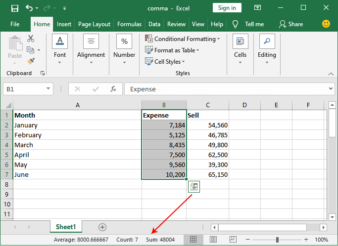
Sum of Sell columnNow, see the total sum of one more column, i.e., the Sell column. You can see the total sum of the selected column (Sells) at the bottom in the status bar. Sum = 318095 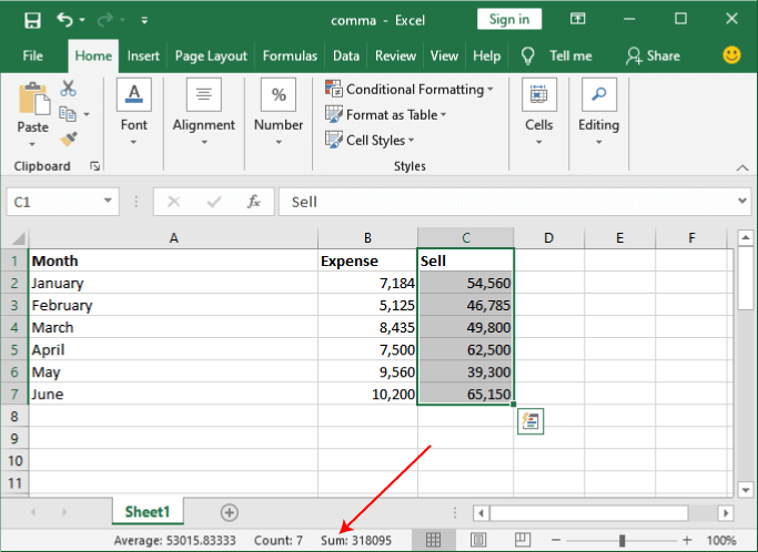
Total the sum of a column using AutoSumAutoSum is another way to find the sum of a column in an Excel spreadsheet. This method is helpful when you want to keep the result in your Excel table for future use. You can use this AutoSum function of Excel. Note: The user can use this calculated sum result in the future when need because Excel keeps it.AutoSum is also an easiest way to total the sum of a column when you want to keep the result. Let's see how this AutoSum function is used in Excel and how it works - For Example We have an Excel spreadsheet containing some products with their price list. We will calculate the total price of these products using the AutoSum function. Follow the steps below: Step 1: Select an empty cell just below the column for which you would like to calculate the total sum. 
Step 2: Now, go to the Formula tab, where click on the AutoSum button present inside the Function Library section in the Formula tab. 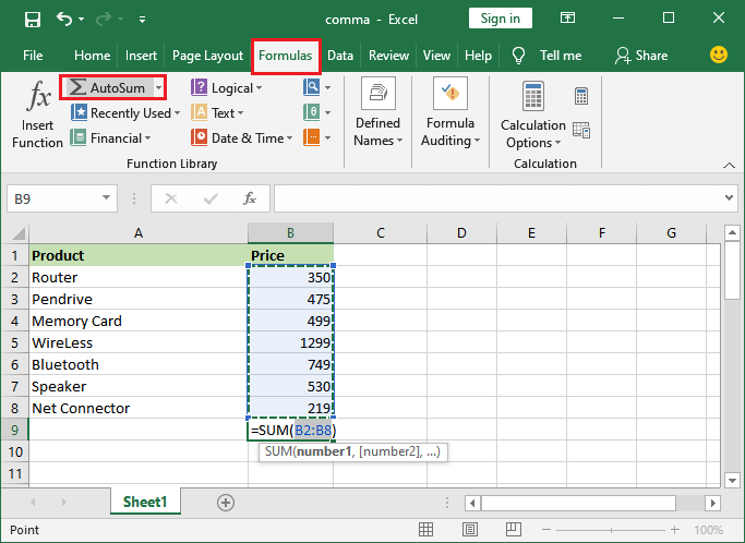
Step 3: Press the Enter key to complete the action and display the calculated sum of Price column. The sum for that column will be automatically calculated and pasted in the selected cell. 
There was no range selection while calculating the sum for the Price column. We have summed the column for all values. Apply the Sum() function to a column manuallyYou can also apply the Sum() function manually to a column instead of an automatic sum. The Sum() function enables the user to calculate the sum manually by applying it to column data. Like the AutoSum function, it also keeps the result of the sum in your Excel table. You are thinking that what is the main objective of applying the Sum function manually and how it is different from AutoSum? Using this function, one can total the sum for the selected cells instead of all values of the column and paste the calculated result anywhere in the Excel sheet. Purpose Sometimes, we require calculating the sum manually if we want to calculate the sum of few selected cells. Use the SUM() function of Excel manually and find out the sum for the selected cells or a range of cells. Let's see how this Sum function apply to a column manually and how it works - For Example For this example, we will use the same Excel spreadsheet used in the previous method containing some products with their price list. We will calculate the total price of these products using the Sum() method. Follow the steps below: Step 1: Click on an empty cell where you would like to paste the total sum of the selected cells. 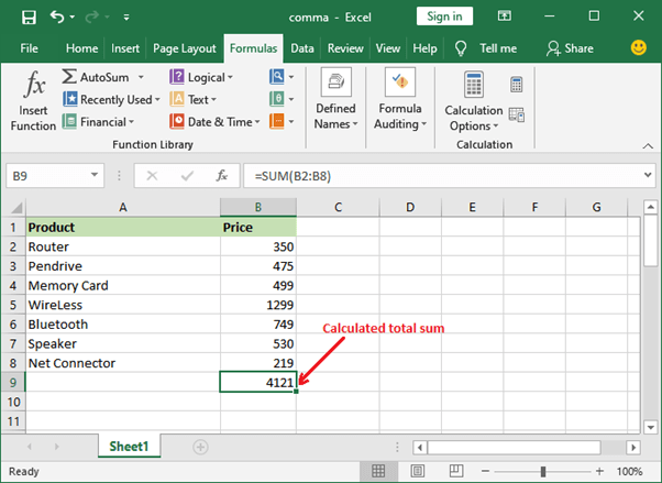
Step 2: Use the following formula of SUM For Example =sum(B2:B11) It will total sum the data from B2 cell values to B11 cell. 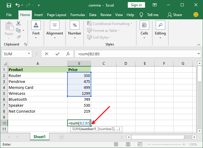
Tip: You can use the range in Sum() formula like (B3:B5000) for the large range of calculation. Step 3: Now, press the Enter key to get the result. See that the total sum for the selected cells (from B2 to B5) has been pasted below. 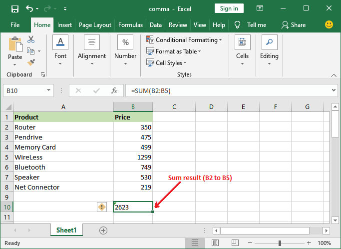
Here, you see a yellow color error type symbol, indicating to that the formula used for this cell apply to the range of cells. 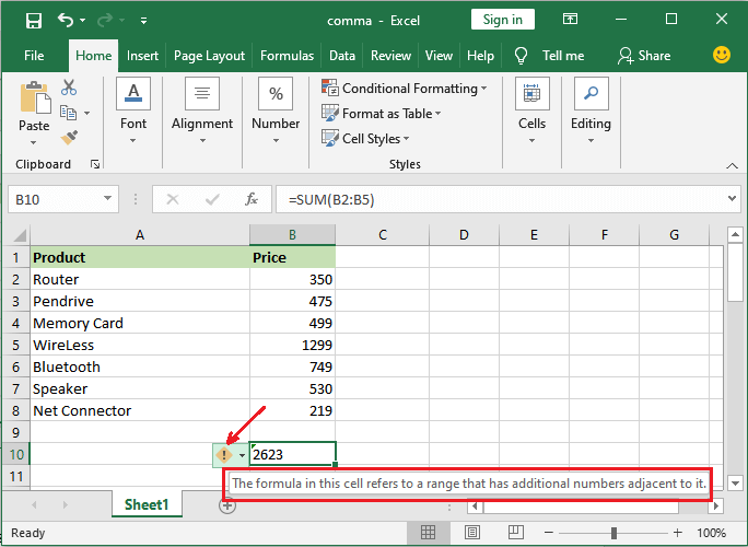
In the Formula bar, you can see the formula applied to the resultant cell. Note: SUM() function can work even for hidden and filtered row data.Use Subtotal to calculate the sum for selected cellsSubtotal is a bit different than Sum function. Subtotal is a mathematical function used to calculate the sum only for the visible cells. Unlike the Sum() method, it does not include hidden or filtered rows data while totaling the column data. Subtotal function only totals the sum of visible row data of a column. It has a bit complicated steps to see the full functionality of this function. Otherwise, it is as easy as other functions (Sum, AutoSum) used above. We will brief you each step. We will use this table data for the Subtotal function: 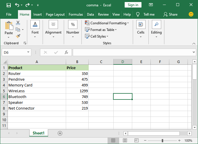
Add filter to the table To show you the actual use of the Subtotal function, we will first filter the table data based on some conditions. For instance, we will add a filter on the Price column and filter the table data by putting greater than condition, e.g., greater than 350. Step 1: Open an Excel sheet to filter the data and go to the Data tab. 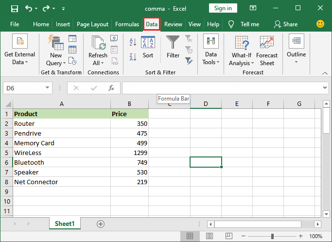
Step 2: Firstly, click on a valid column and then click the Filter icon to add the filter button on each column of the table. 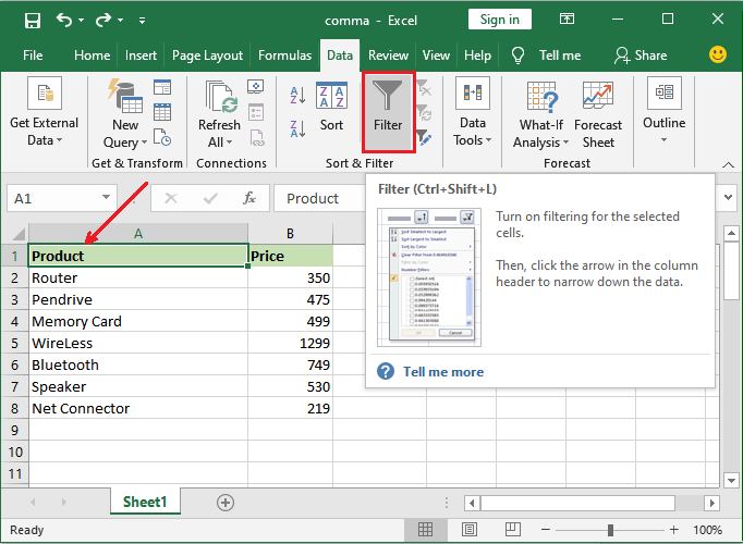
Step 3: These added filter buttons will allow you to filter the data by putting conditions. You will see that a dropdown arrow is added to each data column. 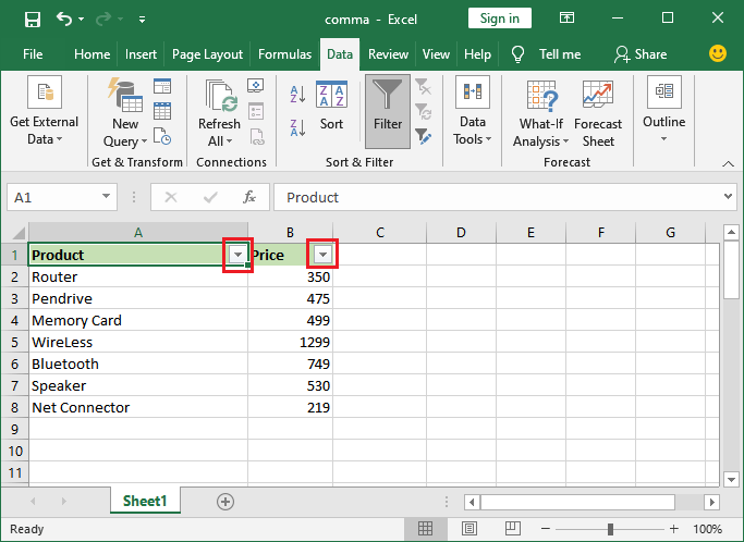
Note: These filters enable separate t filters for string and number type column values.Step 4: Click on this filter dropdown list and choose explore the Number Filters option here. We have clicked on the Price filter button. 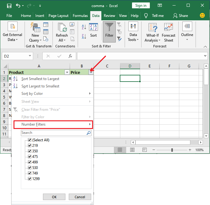
Step 5: Choose a condition from the Number Filters to filter the data. We will choose greater than condition to filter the table data. 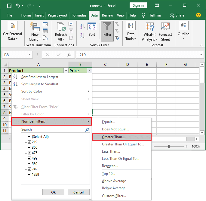
You can also exclude any row from here by unmarking price column data. Step 5: When you will choose any number filter from here, it will open a panel to provide the value to it. Provide the value here to filter the table data and click on the OK button to apply the filter. 
Step 6: After applying the greater than filter on the Price column, you will see that table data has been filtered. The rows having greater than 450 price of product are visible. 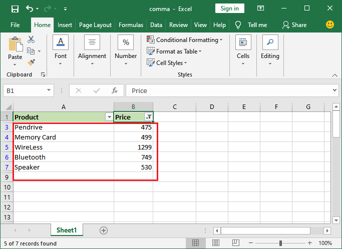
The rows having less than 450 price of the product are hidden by the filter. Use AutoSum function to Subtotal a column dataWe will now sum a column data using the AutoSum function, but after applying the filter. Only then will it work as a Subtotal function. This time it will not include the hidden or filtered data that is not visible currently. Follow the steps to Subtotal a column data: Step 7: Select an empty cell just below the column for which you would like to calculate the total sum. 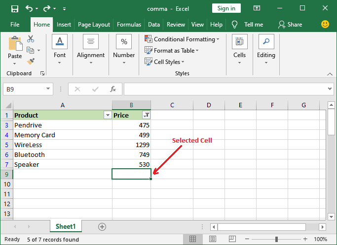
Step 8: Now, go to the Formula tab, where click on the AutoSum button present inside the Function Library section in the Formula tab. 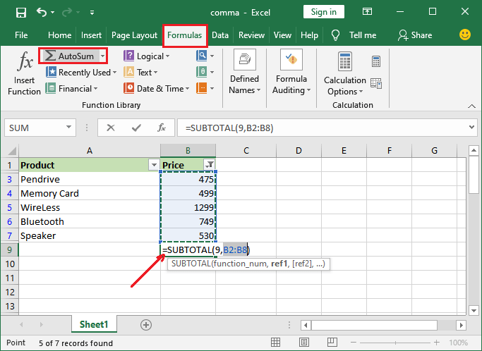
Step 9: Press the Enter key to complete the action and display the calculated sum of the Price column. The sum for that column will be automatically calculated and pasted in the selected cell. 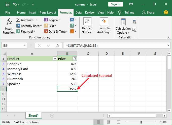
Here, Excel will keep the result. But if you just want to see the total of visible cells and do not want to keep the result, you can select the range of data in a column and see the sum in the status bar. Convert the data to Excel to get the sum of a columnIt is another method to get the sum of a column in an Excel spreadsheet. If you often require to sum a column, you can convert the spreadsheet to an Excel table. It makes it easy for the users to totaling the columns as well as rows. It also allows you to perform some other operations on this list. Follow the below steps how it will be done: Step 1: Press the Ctrl + T shortcut key to format the range of cells of an Excel table. Simply says that it will create a table of your spreadsheet. It will open a Create Table panel window. 
Step 2: Click on the OK button here on this Create Table panel. 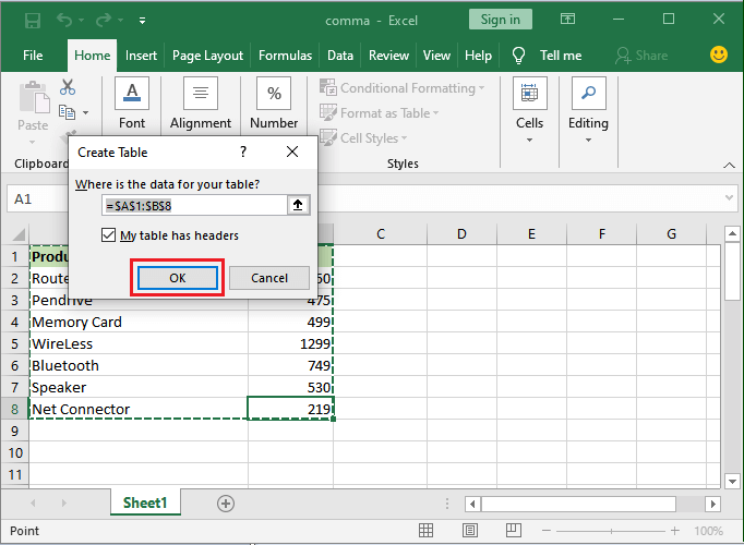
Step 3: A new Design tab will appear in the Excel menu bar; navigate to this tab. In this Design tab, mark the Total Row checkbox inside the Table Style Options. 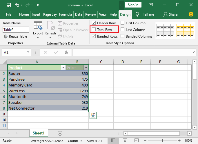
Step 4: A new row will be automatically added at the end of the Excel table when you mark the Total Row checkbox. This row will contain the sum of all the present in this table. 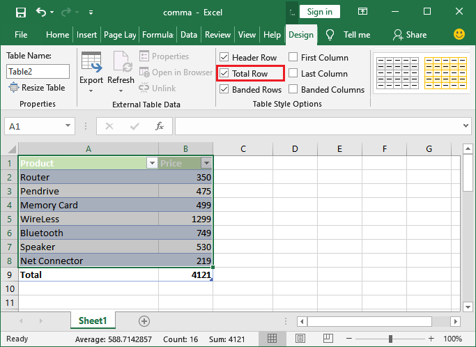
Step 5: To ensure that the resultant data is the sum of rows, click on that resultant number, like 4121 here, that will enable a small down arrow button near/next to this. 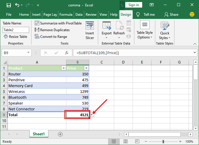
Step 6: Click on that small down arrow button. You will let what you get from this method, such as - sum, min, max, average, etc. By default, the sum is always calculated, as you can also see in the below screenshot. 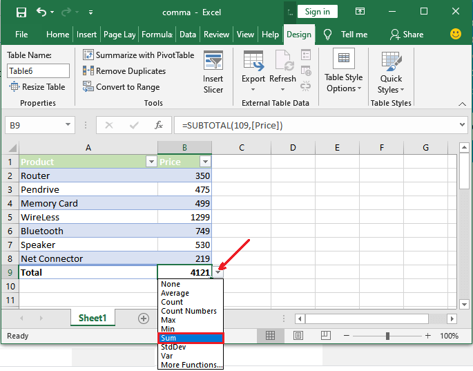
Using this option, you will let the total for each column. Step 7: Similarly, choose any other operation from the down arrow dropdown list, like Max, to find out the max value present in this column. 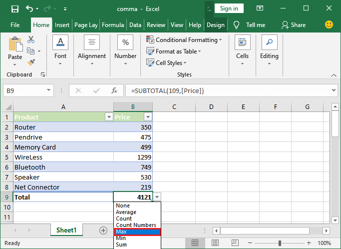
Step 8: See that the maximum value of the column has appeared here. 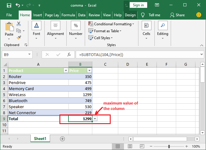
Similarly, you can also find the sum, min, max, or average value for this column by selecting the respective operation from here. Sum a column values based on criteria using SUMIFApart from all these methods discussed above, we have one more conditional method to sum a column value. These methods gave the sum of a whole column except the Subtotal method. Sometimes, a user requires totaling the values that satisfy a condition set by the user. Thereby, we will brief you one more Excel function to sum column values based on a condition. SUMIF is a function used in an Excel spreadsheet to total a column value by applying some conditions. This function helps to total the column data only, which satisfies the defined criteria. You can easily do it using the SUMIF method. Let's understand with an example - Example 1: SUMIF We have a dataset of products and their price. We will calculate the sum of all products whose price is greater than 550. Use the following SUMIF formula and get the total of the cells which satisfy the defined condition. Follow the steps to calculate sum using the SUMIF function: Step 1: Open your worksheet, select the cell where you want to paste the result. 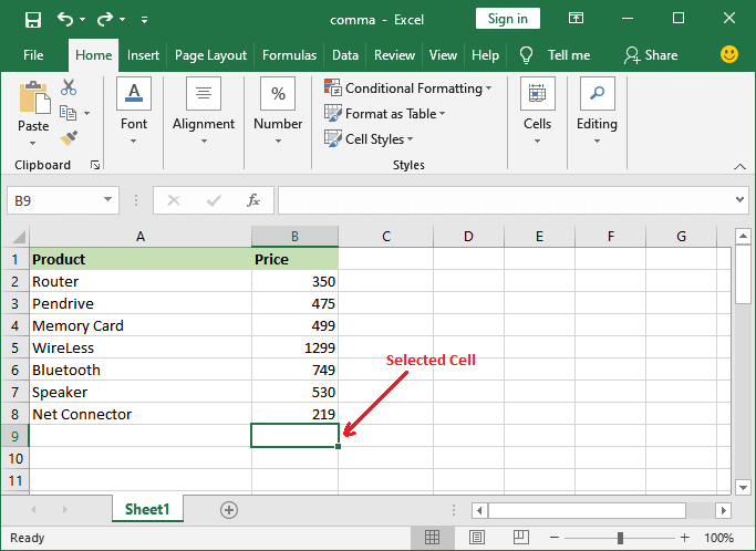
Step 2: Go to the Formula bar and paste the above formula in it. 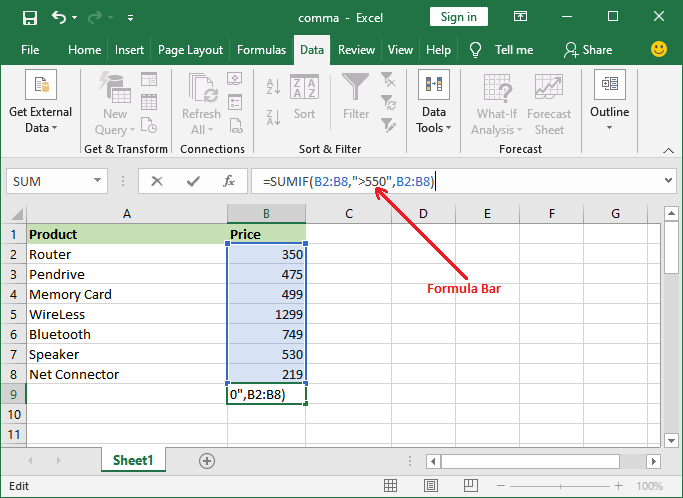
Step 3: Press the Enter key to get the result. 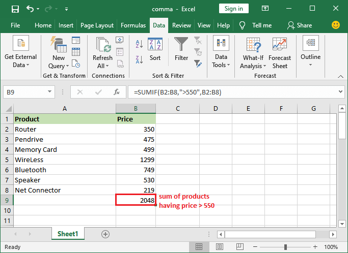
Note: You can use the SUMIF formula on numeric as well as test conditions.Suppose we have to calculate the total sum of all pen drives present in this spreadsheet. In that case, use Pen drive as a condition and include both A and B columns. i.e., Product and Price. Example 2: SUMIF Copy and paste the following SUMIF formula in the formula bar: 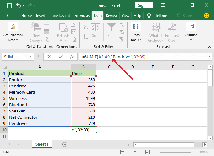
Press the Enter key and get the total prices of pen drives present in this Excel spreadsheet. 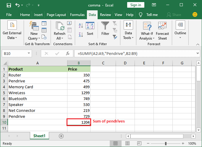
Besides that, SUMIFS is another function that is almost similar to the SUMIF.
Next TopicHow to remove the filter in Excel
|
 For Videos Join Our Youtube Channel: Join Now
Feedback
- Send your Feedback to [email protected]
Help Others, Please Share


