Excel Charts: Tips, Techniques, and Tricks

What is a chart?

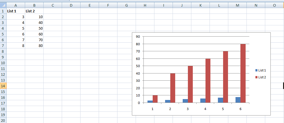
The chart is defined as the graphical representation of data in various forms, such as Pie charts, bar charts, line charts, etc., based on the data and type of preference. It represents the data in an attractive and organized manner which helps the user to conclude the result and make decisions easily and quickly.

Why is data represented in the form of a chart?

The data is represented in the form of a chart for the following reasons:

• Defining the data in a chart helps to understand the data easily and quickly.
• The pictorial representation of the chart makes the data attractive and easily understandable.
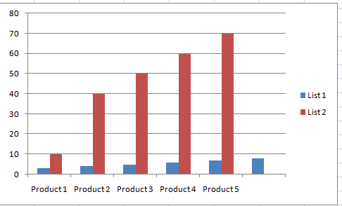
• It helps the user to compare various values. For example, if the data is based on sales reports of the year based on multiple products, to quickly analyze each product, representing the data in the form of a chart help to compare easily.

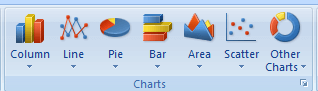
Types of Charts in Excel

The various types of charts present in Excel are described as follows:

1. Column Chart: The column chart represents the data as a vertical bar.
2. Bar Chart: The bar chart illustrates the data as a horizontal bar.
3. Line Chart: It displays the trends in the data represented in the form of data points connected using a continuous line.
4. Pie Chart: The pie chart is represented in the form of a circle that contains various slices. The size of each piece represents the proportion of the whole.
5. Area Chart: It is represented in the form of a line chart. The area below the line is colored or shaded. It helps the users identify the product changes based on time.
6. Scatter Chart: The scatter chart represents the data in two-dimensional graphs. The users can compare the values in the chart.
7. Bubble Chart: It represents the data in a bubble similar to a scatter chart. The size in the bubble chart indicates the value of the third variable.
8. Stock Chart: As the name suggests, it displays the various aspect of the chart, such as increasing and decreasing the day's price.

The chart is chosen for displaying the data based on the user's choice and data.

How to save an Excel chart as a Picture?

The user can save the Excel chart as a picture which helps to insert it in various files or web in the future. The document is saved as a picture which is available for future records. To keep the Excel chart as a picture, the steps to be followed are:

1. Open the required worksheet, which contains the chart for the required data.
   
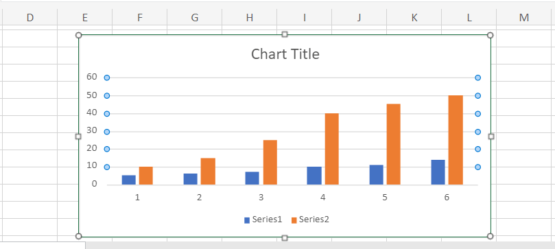
2. Before saving the File, bring the chart to the required size to be protected.
   
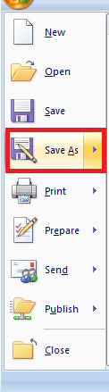
3. Choose File>Save As option. In that, choose the appropriate location to save the File.
   
4. Enter the required file name, and in the "Save as Type "dropdown list, choose the option Web Page.
   
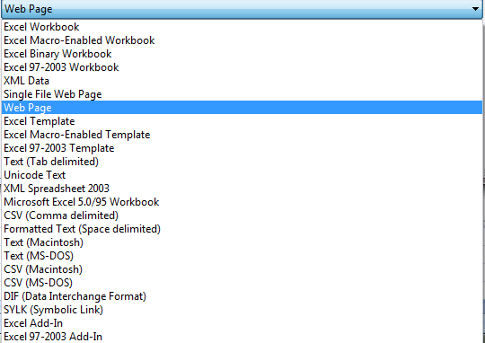
5. Click Save.
6. This converts the worksheet into html file. The html file doesn't contain images. Hence the chart is saved separately and linked with the html file.

For example, if the File is saved as stock market.htm, the images will be stored in the File in the name of stock market_files. It is stored in a PNG file.

Note: The Excel workbook must be saved in the required name for future reference and usage.

How to adjust the column overlap and spacing in the chart?

To make the chart professional and attractive, the chart needs to be edited and modified. Increasing the gap between the columns in the chart makes the data more visible.

The steps to adjust the column overlap and spacing of the chart are to be followed:

1. Open the required worksheet containing the chart for the given data.
   
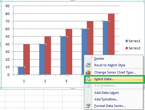
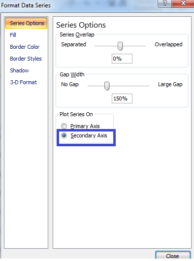
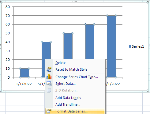
2. Right-click the chart and choose the option Format Data Series.
   
3. Drag towards the separated or overlapped option in the Series overlap option based on the requirement. To increase the spaces, choose the Overlap option.
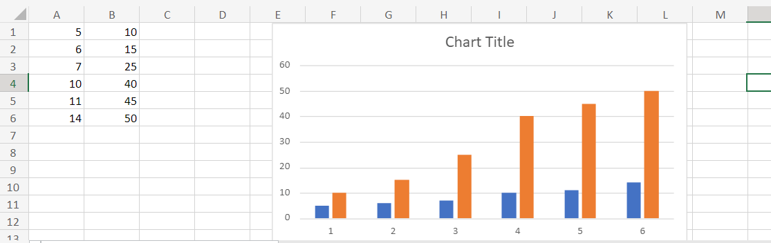
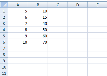
   For example, if two charts contain the data, the smaller chart is behind, the larger one. To change the chart type, right-click the data and click Select data.
   
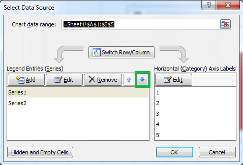
4. The Select Data Source dialog box will open. In that, choose Series 1 or Series 2 based on the larger or smaller data.
5. Click the Move Down button in the dialog box that needs to be placed behind the larger series.
6. These changes will present the smaller data series before the larger data series.
   

Plotting the date-based data in the chart

While plotting the chart based on the date, the bar is narrow. To change the Format of the X-axis, right-click towards the X- axis.

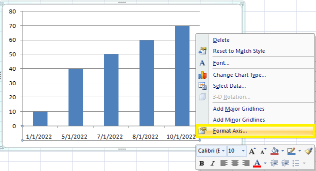
1. In the option, click the Format Axis option.
2. In the Format Axis dialog box, choose the Axis option.
3. In the Axis type, select the Text Axis among the various options.

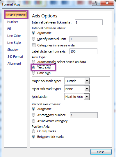
Choosing the option makes the X-axis wider, and if more space is needed, the user can adjust it based on preference.

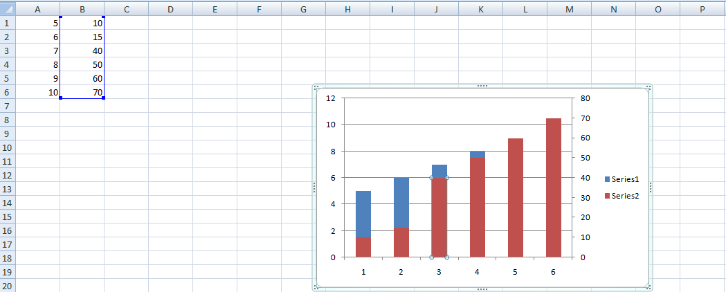
How to plot a second axis?

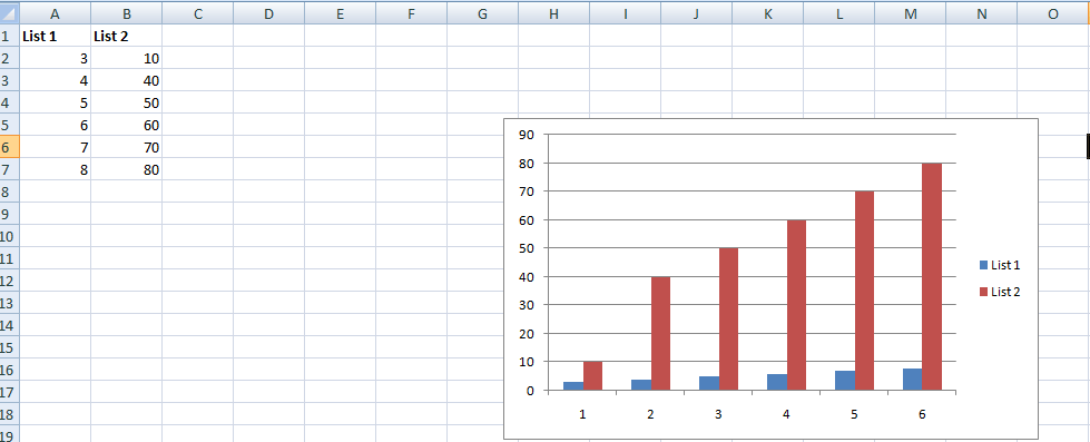
Usually, the project contains multiple data, and if larger data are plotted while plotting the smaller data, it is invisible, which is present behind the bar. For example, to plan the percentage among millions, the steps to be followed are:

1. Open the worksheet containing the chart for the data.
   
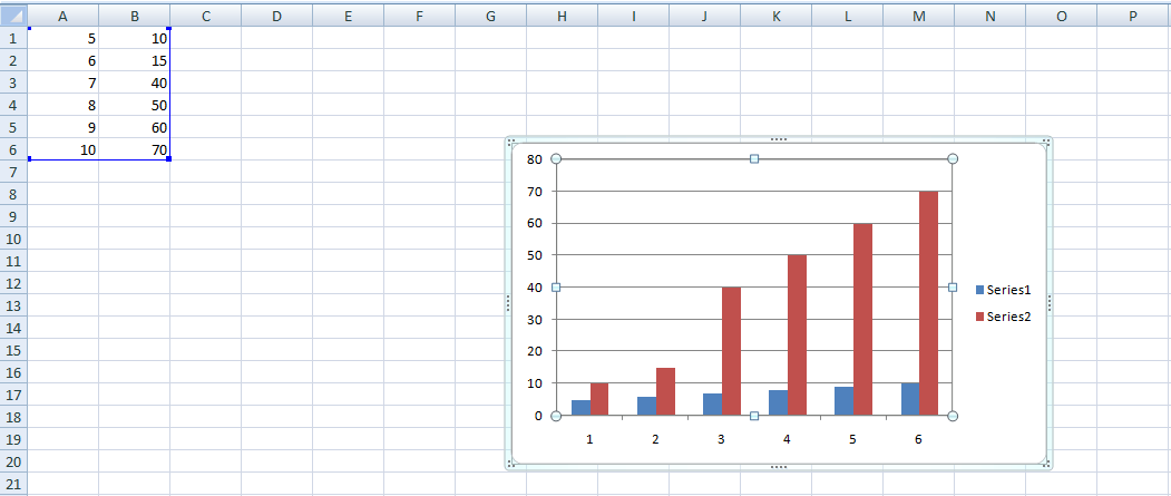
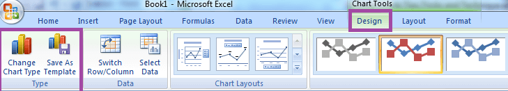
2. Right-click the chart and choose Chart Tools>Layout tab.
   
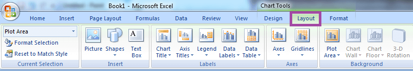
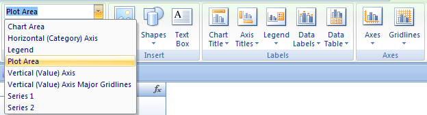
3. Select the difficult series in the chart element sector in the top left corner.
   
4. In the format selection group, click Secondary Axis and Close.
   
5. Next, select Chart Tools> Design Tab and choose Change Chart type.
   
6. Now a different chart type-like line is selected.
   

How to create a combination chart?

Creating a combination of charts is useful to make the data more understandable and clear. The user can create the combination chart if they are required. To create a combination chart, the steps to be followed are:

1. Open the required worksheet containing the data for the chart.
   
2. Insert the first chart type, such as the column chart.
   
3. Select the series for the required chart type, like line chart, etc.
   
4. Select the second chart type by clicking Chart tools>Design tab>Change Chart Type.
   
5. A combination of certain charts are not combined, such as bar charts and column charts, but charts like line and column charts will be integrated.
   

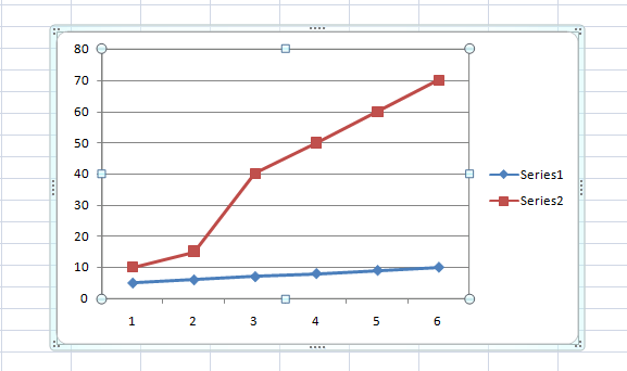
Chart as Table

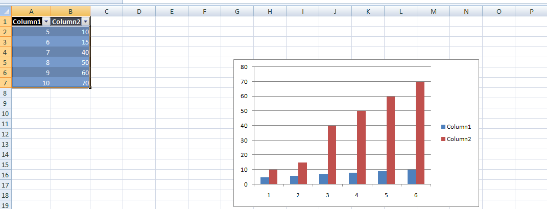
Every time the user enters various data. Each data has a different specification. Hence inserting the chart is based on the data. Sometimes the data may grow based on time. For such data type converting the chart to a table helps to add more data. The steps to correct the chart as Table as follows:

1. Open the worksheet which contains the required data.
   
2. Select the data, and choose Format as Table in the Home tab from the Ribbon tab.
   
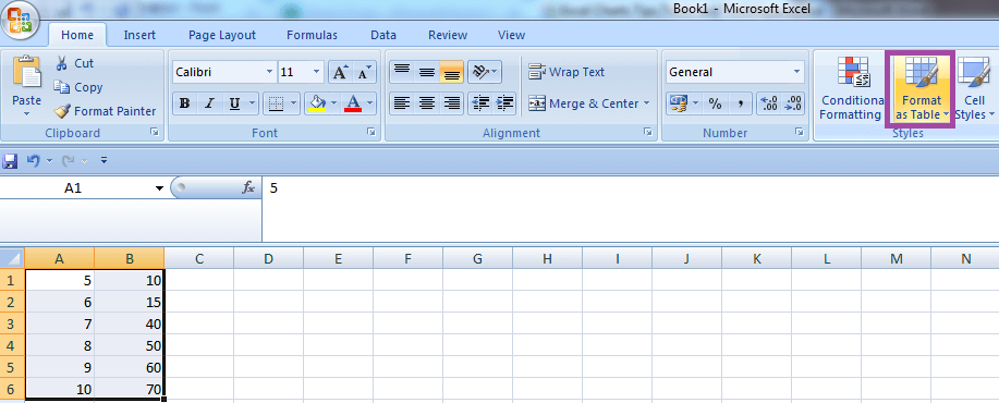
3. Now the data is formatted as a table, and the chart is based on the Table. If new data are added to the Table, it also increases the data in the graph.
   

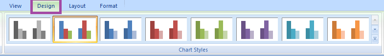
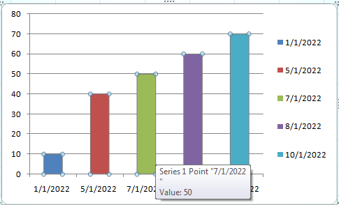
How to apply various colors to the data present in the chart?

When the data is plotted in the chart, the color for the entire bar is the same. To apply various colors for the data present in the diagram, the steps to be followed are:

1. Open the worksheet that contains the chart for the required data.
2. Right-click the chart and choose Format data series and click the Fill option.
   
3. The Format Data Series dialog box will open. If the data is based on one series, choose Fill> Vary Colours by point.
   
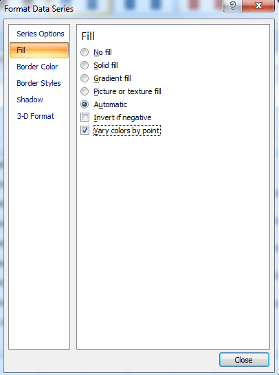
4. It fills the various colors for the column bar in the chart.
   

Note: If the chart contains one or more series, to apply specific color for the data point, click on the individual data series, right, click choose Format data points.

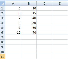
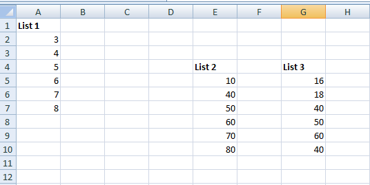
How to chart non-contiguous data?

The data entered by the user, sometimes not lined up in a column side by side, to chart the graph in an organized way. The steps to be followed are:

1. Open the worksheet containing the required data.
   
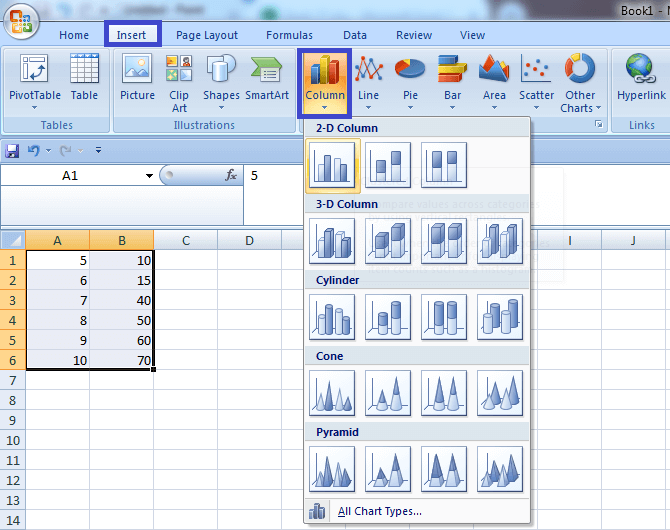
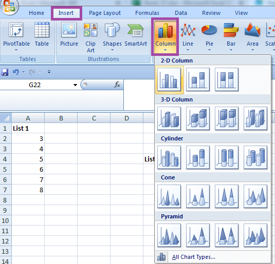
2. Insert a blank chart by choosing the Insert option in the Home tab in the Ribbon group. Here column chart is selected.
   
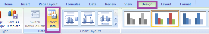
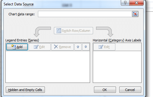
3. Click on the blank chart, choose the Design option in the Ribbon tab, and click Select Data.
   
4. The Select data source dialog box will appear, and choose the option Add.
   
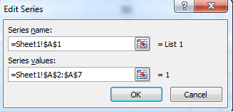
5. After clicking the Add button, the Edit Series dialog box will open. In that, enter the required Series name and Series Value.
   
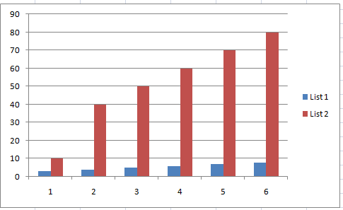
6. The chart for the selected data will display in the worksheet. Repeat steps 4 and 5 to insert the various data in the chart.
   
7. After inserting the required chart, click the Edit option in the Select data source dialog box. The information for the Horizontal Axis Label is added.
   
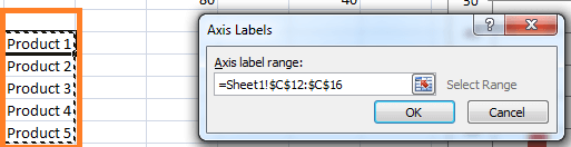
8. After entering the data, click ok. The chart for the non-contagious data is created successfully.
   

How to save a chart as Template?

By saving the chart as a template, the user can use it whenever needed, based on their desired Format. To create the chart as a template, the steps to be followed are:

1. Open the required worksheet containing the graph.
2. Design the desired chart based on the requirement.
   
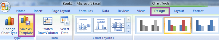
3. Select the chart, choose Chart Tools>Design tab, and choose the option Save as Template.
   
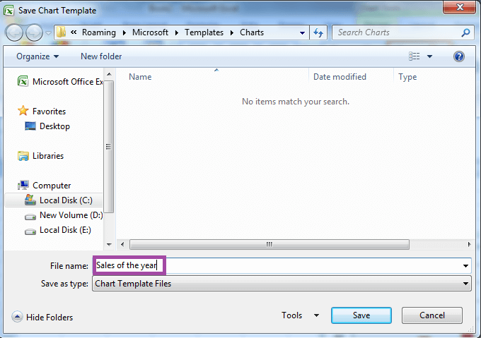
4. Name a chart and click the save option.
   
5. Now the design of the chart is saved. If the user creates the chart for the data, the creation of the saved chart is used. To use the product of the existing graph,
6. Click the chart, choose Chart Tools>Design tab, and click Change Chart type.
7. The Change Chart Type dialog box appears in that choose the option Templates.
   
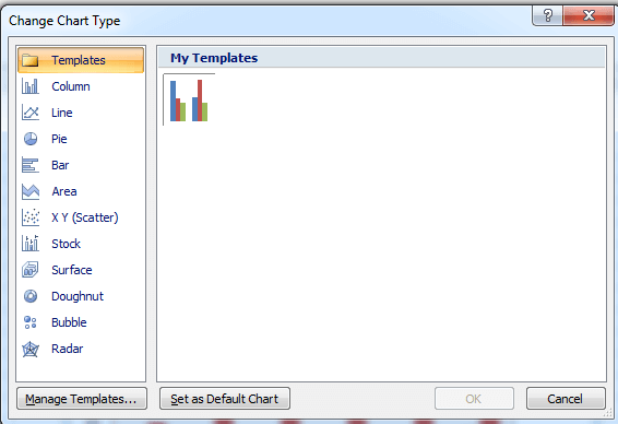
8. Select the required template option and click ok.

Note: The Excel template chart can be saved as a favorite chart used for future projects quickly whenever the user is needed.

How to enter a smarter chart title?

The user can set the chart title to the desired cell in the worksheet. To put the chart title in a cell, the steps to be followed are:

1. Open the worksheet containing the required data and chart.
   
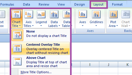
2. Set the required chart title, which is placed above the respective position, by selecting the option Chart tools> Layout tab> Chart title.
   
3. Select the chart title, where a chart title with a box is displayed after selecting the title.
4. Now choose the formula bar in the ribbon bar and type the cell reference where the title needs to be placed in the cell.
   
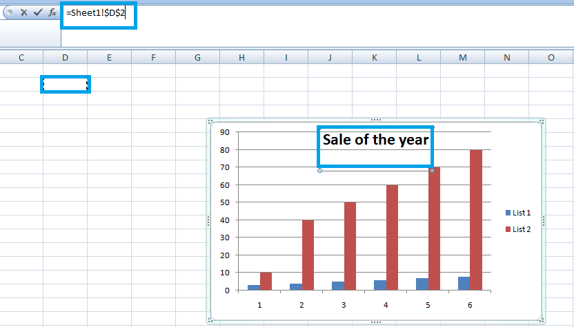
5. The user can also add the Sheet name before the cell reference. For example, if the sheet contains the cell title in cell D2, the sheet name is added before the cell as follows =Sheet 1! $D$2.
6. The title will change if the contents of the cell are changed.

Summary

Creating a chart for the data helps in various ways, such as understanding the data clearly and quickly, decision-making, analysis, and organizing the data. The user creates the chart based on the different requirements in data. This tutorial explains the various tricks, techniques, and trips for creating the chart.