Excel SUBSTITUTE FunctionReplacing a text with some other text is a common job that we all do in Excel, and we all have different ways to do so. But do you know that Excel has provided an inbuilt function named SUBSTITUTE to replace one or more instances of text strings with another. In this tutorial, we will take a deeper look at the SUBSTITUTE function. What is SUBSTITUE function?The Excel Substitute function replaces a part of the text in a string with some other text. SUBSTITUTE function is used to clean data by substituting one or more characters from imported data. For example, if we have imported some data from a PDF file in a format 458-299-605, we apply the SUBSTITUTE function to transform it into 458299605. The Excel SUBSTITUTE function replaces or substitutes the text strings with other text strings. You can use the SUBSTITUTE function to replace the text based on matching (remember, it doesn't work with position). You can also replace one or more text strings with no data; you need to pass an empty string ("") in the argument. SUBSTITUTE is an inbuilt function categorized under Excel Text Functions. SUBSTITUTE function is case-sensitive. You can use it as a worksheet function in Excel. The SUBSTITUTE function can be inserted as part of another formula in a cell as a worksheet function. This function allows you to substitute the text in strings easily, and it gives you the ability to decide which part of the string you want to replace. The alternative option of this function is to use the Find and Replace Excel feature. NOTE: A single SUBSTITUTE function can only replace one text value at a time. However, you can nest the SUBSTITUTE function inside of itself to replace more than one string.\SyntaxParameters
Points to Remember for SUBSTITUTE function
Example 1: Use SUBSTITUTE function to make changes to some of the strings below to get the results mentioned in the 'Result' column.
To SUBSTITUTE you data follow the below given steps: STEP 1: Add a helper column named OutputPlace your mouse cursor to the cell next to "Result" and name the new column as "Output". It will look similar to the below image: 
We will type our SUBSTITUTE formula in this column and place the SUBSTITUTE data for different text values. NOTE: Format the helper column and match it with the match column to make your Excel sheet more attractive.STEP 2: Type the SUBSTITUTE formulaPut your cursor to the second row and start typing the function: = SUBSTITUTE( It will look similar to the below image: 
STEP 3: Insert the parameters
Our final formula will look similar to the below image:
STEP 4: SUBSTITUTE will return the resultThe SUBSTITUTE will replace the character "b" with "t" and will return the output as "Bot". It will look similar to the below image: 
STEP 5: Repeat the formula for the other rows
Refer to the below image for all the outputs: 
That's it, and now you have successfully learnt how to use the SUBSTITUTE function in Excel. Let's explore some complicated examples. Example 2: Demonstrate the use of nested SUBSTITUTE function using below table: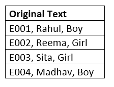
The SUBSTITUTE function cannot replace more than one string in a single function. Since in the above table, we have to replace all the three strings, we need to have three separate SUBSTITUTE functions in the same cell and get three of them replaced. To achieve this, the best method is to nest ONE SUBSTITUTE function inside other. To understand nested SUBSTITUTE functions follow the below-given steps: STEP 1: Add a helper column named SUBSTITUTE OutputPlace your mouse cursor to the cell next to "Original Text" and name the new column as "SUBSTITUTE Output". It will look similar to the below image: 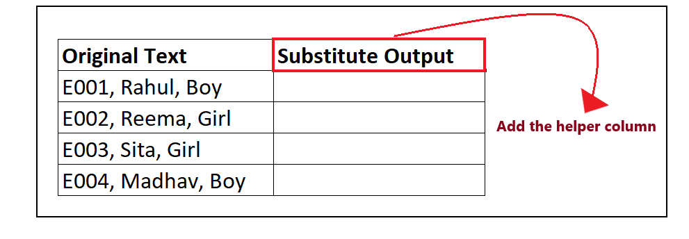
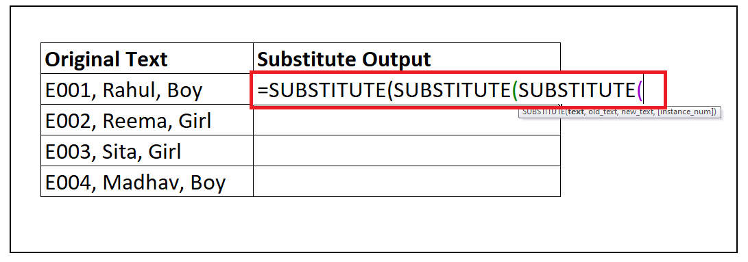
We will type our SUBSTITUTE formula in this column and place the SUBSTITUTE data for different text values. STEP 2: Type the SUBSTITUTE formula
STEP 3: Insert the parameters of the nested substitutes
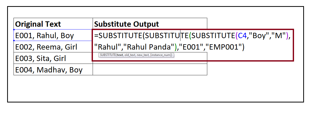
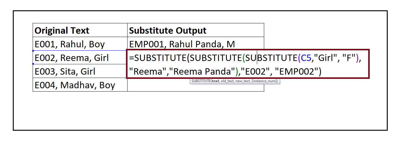
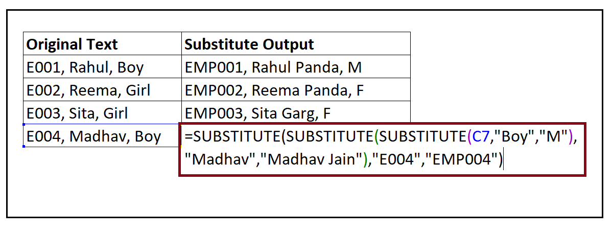
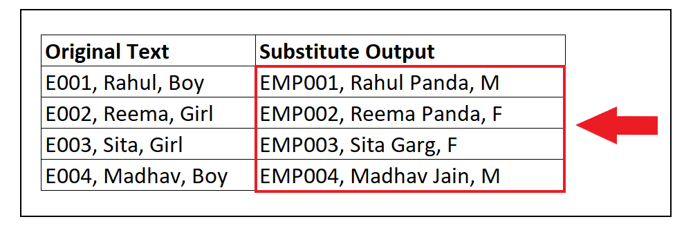
=SUBSTITUTE(SUBSTITUTE(SUBSTITUTE(C4,"Boy","M"),"Rahul","Rahul Panda"),"E001","EMP001") Our formula will look similar to the below image: STEP 4: SUBSTITUTE will return the resultThe nested SUBSTITUTE functions will replace all the old strings with the new strings and will return the data at once. The output will look similar to the below image: STEP 5: Repeat the above formula for the following rows
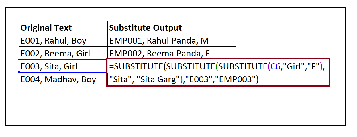
It will replace all the Old_Text with the New_Text and give you the result. The nested SUBSTITUTE functions will replace all the old strings with the new strings and will return the output for all the rows. Refer to the below image: Example 3: Using the SUBTITUTE function remove the line breaks from your Excel worksheet.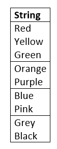
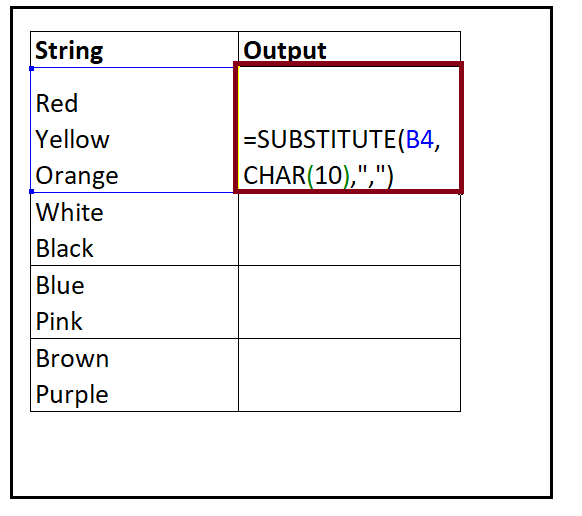
To replace the line breaks from the text, you can use a combination of SUBSTITUTE and CHAR functions. To remove the line breaks from your cells follow the below-given steps: STEP 1: Add a helper column named SUBSTITUTE OutputPlace your mouse cursor to the cell next to "String" and name the new column as "Output". It will look similar to the below image: 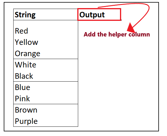
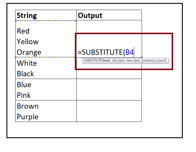
In this column we will type our SUBSTITUTE formula and place the SUBSTITUTE data for different text values. STEP 2: Type the SUBSTITUTE formulaPut your cursor to the second row and start typing the function = SUBSTITUTE( It will look similar to the below image: 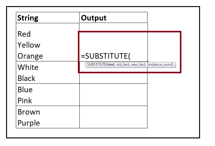
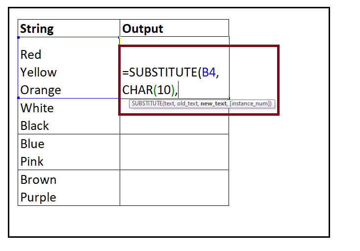
STEP 3: Insert the parametersSUBSTITUTE can locate matching text anywhere in a cell and replace it with the text of your choice. SUBSTITUTE can accept up to four arguments, but we will use only the first three and skip the fourth parameter.
Refer to the below image: STEP 4: SUBSTITUTE will return the resultThe SUBSTITUTE function will replace all line breaks or Char (10) characters with comma (,) from B4 cell and will return the final output i.e, "Red, Yellow, Orange" in cell C4. Refer to the below image: 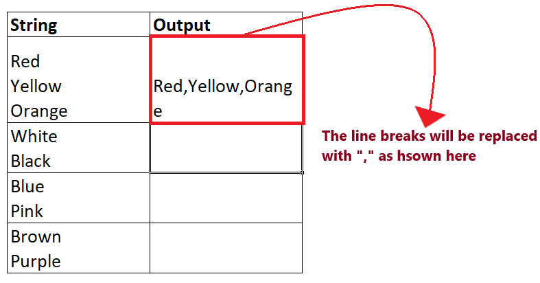
STEP 5: Drag the formula to other rows to repeat
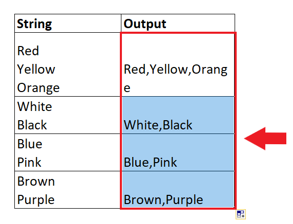
Next TopicSpecial Symbols in Excel
|
 For Videos Join Our Youtube Channel: Join Now
Feedback
- Send your Feedback to [email protected]
Help Others, Please Share


