XLOOKUP VS INDEX-MATCH IN MICROSOFT EXCEL

It was well known that, in the realm of Microsoft Excel data management, two powerful functions stand out for their proficiency in searching as well as retrieving information: XLOOKUP as well as INDEX-MATCH. These particular functions serve as indispensable tools for Microsoft Excel users who are seeking efficient as well as flexible solutions for effectively handling data lookup operations.

XLOOKUP: A Modern Approach

XLOOKUP is primarily considered a relatively recent addition to Excel's repertoire and was introduced with Excel 365 and Excel 2019 as well. More often, this function is basically designed to simplify the often-complex task of searching for a specific value within a range and returning a corresponding result. XLOOKUP is particularly adept at handling both exact and approximate matches, making it a versatile choice for various scenarios.

This function's strength lies in its streamlined approach, thus providing users with an intuitive way of handling lookups. It mainly accepts the lookup value, the range to search for this value and the corresponding range from which to return results. An optional parameter allows users to specify a value or the action if the lookup value is not found. More often, the respective XLOOKUP's function has the ability to handle out the approximate matches with the ease to add to its appeal, mostly in the case where there is an involvement of the numerical as well as the ranges in the data.

INDEX-MATCH: The Classic Duo

And it was well known that, the respective INDEX-MATCH primarily relies upon the combination of the two established functions, with its distinct rule, and also, the MATCH function firstly determines out the position of the lookup value in the specified range, and the INDEX function subsequently retrieves the corresponding value from other range as well. This pairing provides a more granular level of the control, especially while dealing with the datasets where a direct vertical lookup is not practical. Moreover, the ability to handle non-contiguous data effectively is a hallmark of the INDEX-MATCH combination, thus making it a preferred choice for users accustomed to its flexibility.

However, the decision between the XLOOKUP and the INDEX-MATCH more often depends upon the specific needs of the task at hand. The XLOOKUP is favored for its simplicity and ease of use, and with this making it an excellent choice for the users who prioritize a straightforward approach to the lookups. Its support for the approximate matches is particularly beneficial while dealing with the large datasets or ranges where an exact match may only sometimes be feasible.

And the INDEX-MATCH usually shines in situations that mostly demand a more intricate approach. Its flexibility allows users to navigate through the complex data structures easily and to perform lookups that may be challenging with other methods as well.

What is XLOOKUP function in Microsoft Excel?

XLOOKUP, is considered to be a relatively recent addition to Microsoft Excel that was introduced in the year 2020, and it revolutionizes the way users search for the specific values in the given dataset. Unlike its predecessors, XLOOKUP offers the flexibility of searching both vertically and horizontally in a table, allowing users to find results to the left or right of the search value in rows and columns. This newfound capability is particularly useful in scenarios where users need to retrieve information based on various criteria as well.

In our provided example, the formula =XLOOKUP (E3, A2: A6, C2: C6) is employed in cell F3 to locate and extract the data. And breaking it down, cell E3 will represent the search value (as in this case, the respective roll number of the student), and the cell ranging from A2:A6 is the Array where Microsoft Excel looks for the value (most often the column containing the roll numbers). The cell ranging from C2:C6 is the Array from which the corresponding result is usually retrieved (the column containing the marks). The result, 49 in this instance, primarily represents the marks secured by the respective student with the roll number 1003 respectively.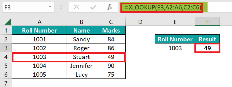

Moreover, this formula essentially communicates to Microsoft Excel: "Find the roll number in column A and then after that returning out the corresponding marks from column C." The introduction of the XLOOKUP streamlines as well as simplifies such search operations, thus making it a powerful tool for users navigating datasets in both professional and personal contexts.

List out the advantages of using XLookup in Microsoft Excel.

It was well known that the respective XLOOKUP is termed to be the game-changer in Microsoft Excel, transcends the limitations of the traditional lookup functions like VLOOKUP or the HLOOKUP, and thus offering a plethora of the advantages that usually streamline out the data retrieval and its analysis. So, let us delve into the key benefits that make the XLOOKUP a powerhouse in spreadsheet applications.

1. Bidirectional Search Capability: XLOOKUP primarily stands out with its ability to search both vertically and horizontally as well, and this bidirectional search flexibility surpasses the unidirectional constraints of the VLOOKUP or the HLOOKUP, thus providing users with a dynamic tool to navigate and also to extract out the data efficiently, regardless of the dataset's structure in an effective manner.
2. Array Return Functionality: A significant advancement is XLOOKUP's capacity to return entire arrays of the values. In contrast to the VLOOKUP, which retrieves only the first match, XLOOKUP usually excels by just delivering a comprehensive range of outputs in a single operation. This proves invaluable when users seek multiple data points that are based upon a single lookup criterion, simplifying complex tasks as well.
3. Unified Handling of Match Types: More often the respective XLOOKUP streamlines the handling of both approximate and also the exact matches within a single function. This eliminates the need for separate functions such as VLOOKUP or HLOOKUP, thus enhancing the efficiency of the formula creation as well as minimizing the errors that are associated with the management of the multiple functions for the distinct match scenarios, respectively.
4. Proactive Error Handling: An impactful feature is none other than the XLOOKUP's ability to specify a value to return if the lookup item is not found. This proactive approach primarily simplifies the management of missing or non-existent data points, fortifying the overall robustness of the spreadsheet models as well as ensuring more accurate as well as reliable results.
5. Intuitive Column Referencing: Moreover, the XLOOKUP function in Microsoft Excel usually eliminates the need to count the columns manually for the "col_index_num" parameter, a requirement in VLOOKUP. This intuitive approach reduces the likelihood of errors stemming from miscounting, enhancing user-friendliness and accessibility.
6. Wildcard Support for Enhanced Flexibility: Introducing the other layer of flexibility, XLOOKUP supports wildcard characters. This capability empowers users to match out the patterns while searching for the values, addressing scenarios where partial matches or specific patterns are very crucial as well. Wildcard support enhances the precision as well as the scope of the data retrieval, providing a nuanced approach to information extraction effectively.

Furthermore, the respective XLOOKUP is termed to be the bidirectional search, array return functionality, unified handling of the match types, proactive error handling, intuitive column referencing, as well as wildcard support, collectively positioning it as an indispensable and versatile lookup function. As users navigate diverse and complex datasets, XLOOKUP emerges as a powerful ally, simplifying the process of finding and retrieving data in Excel while significantly enhancing overall spreadsheet efficiency.

XLOOKUP Function

The syntax that can used for the XLOOKUP function in Microsoft Excel is as follows:

The associated arguments with this syntax are as follows:

• lookup_value - It is the mandatory argument; it is the lookup value that we will retrieve out the result from the Array specified in return_array.
• lookup_array - It is the Array, or the range of the cells searched as well, and it is considered as the mandatory argument respectively.
• return_array - The Array or the range of the cells from which the value is returned, and it is also considered as the mandatory argument.
• [if_not_found] - It is termed to be the text value that needs to be printed if it does not find an exact match in the return_array as well. If this argument is blank, then in that scenario we will be getting a #N/A error if there is no match effectively and it is an optional argument.
• [match_mode] - It primarily specifies the type of the match, and the arguments are quite optional here and the values are as follows:

• [search_mode] - Here in this, we usually specify how to search these arguments is optional as well. The values are as follows:

How can one make use of the XLOOKUP function in Microsoft Excel?

It was well known that the respective XLOOKUP function is an improved version of the VLOOKUP function. Here, it can search a range of cells instead of the respective column effectively. In addition to this, we can manually enter the function in any cell or through the use of the Microsoft Excel ribbon.

1. Entering XLOOKUP In Excel Manually

For this, we can have an Excel sheet that usually contains the names of all eight planets that are available in the solar system as well as their total number of moons in an effective manner.

In this respective example, let us now find out the number of moons of Jupiter.

1. For this, we must look up any planet and then check its number of moons. We can make use of the planet name as the lookup value; the lookup ranges from cell B2 to B9, and the return array from cell C2:C9 as arguments. Enter the formula in cell F4. Here, the first argument is the reference of the lookup value respectively.
   
2. Next, we are required to select the lookup range. As in this case, it will be the planets that are present in Column B. Just after that, we need to select the cells that are effectively ranging from cell B2 to cell B9.
   
3. More often, the third argument is the return array in Column B, which contains the number of moons. And then, we need to select the cells right from cell C2 to cell C9 effectively.
   
4. Now, after performing the above step, we need to close the bracket, and then we need to press the "Enter" button. We need to get the number of the moons of Jupiter in cell F4, which is none other than 80. Note that we have not specified the other optional arguments as we perform a simple search and retrieval effectively.
   

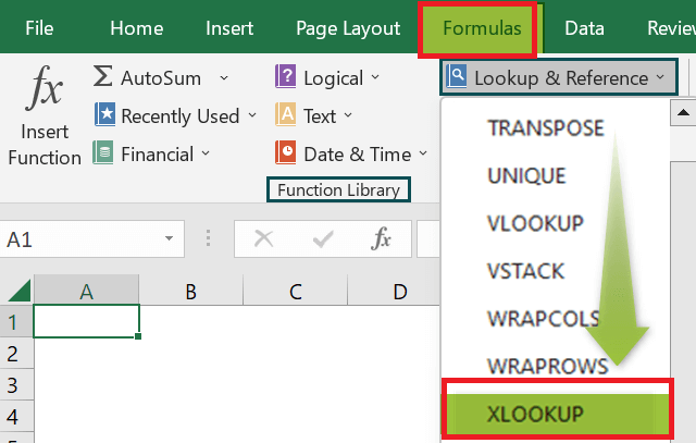
Thus, the function is simple and easy to use when entered manually.

2. Entering XLOOKUP in Excel through the Excel Ribbon

The XLOOKUP shortcut method is to enter it through the Excel ribbon. Then, we need to place the cursor in the cell where we actually need to insert the formula as well.

• And for the purpose of obtaining the XLOOKUP shortcut, we need to go to the Microsoft Excel ribbon, and then we need to click on the Formulas tab respectively.
• Under the "Functions Library," we need to select "Lookup & Reference." Choose the XLOOKUP option as well.
  

And we will be getting a pop-up window where we actually want to enter the arguments respectively.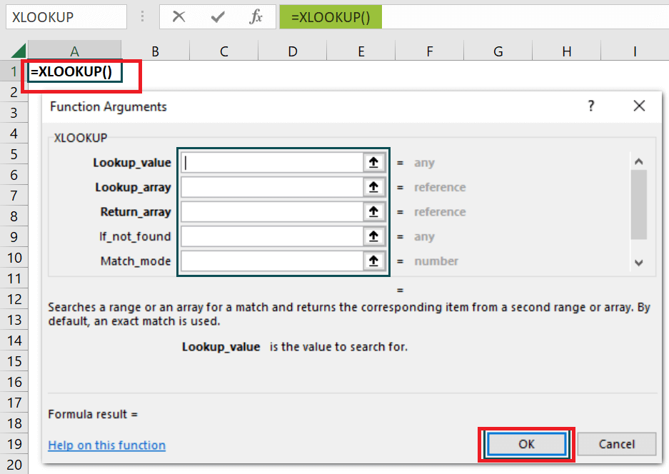

More often, the respective XLOOKUP function can be used in multiple ways, as seen in the examples below respectively.

Examples

The respective XLOOKUP () can efficiently replace the VLOOKUP function with its versatility and ease of use. More often, the examples below depict how to make use of the function to look up any specific values in a given range respectively.

Example #1

Let us now look at how the respective function does an approximate match. So, in the XLOOKUP example below, we have some of the employees' Employee Names in column A and their Salaries, which are stored in column B details. And based on their salary, their Bonus % (Column C) is determined. The range F5:G11 contains the bonus details for different salary brackets.

Step 1:

• Employees who are earning between $ 4,000 to $ 5,000 would get a bonus of 0%. And those who are earning a salary between $ 5,000 to $ 6,000 would get a bonus of 6%, and so on.
• To find an approximate match, we need to enter the fifth argument as -1. Then, it will search for the specified value, and if there is no match, it will return the next smaller value respectively.
• Moreover, an employee who earns $ 5,500 would find and match $ 5,000, the next lower value, and return its corresponding bonus, 6%, respectively.

Just after that, we need to enter the formula =XLOOKUP(B2,$F$7:$F$11,$G$7:$G$11, -1) in cell C2 and press Enter.

Step 2: Just after that, we need to drag the Autofill handle right from cell C2 to cell C9 in order to get the bonus for all the employees in an effective manner.

Example #2

Let us now consider the table below, which contains the names of some different items that are effectively available in the supermarket with their unit price as well. The respective supermarket usually offers discounts on some of its items, which are effectively listed in Columns E and F, respectively.

More often, the respective columns B and G have been formatted as the Currency and Percentage, and just after that, we need to apply the discount percentage to the items that are available in Column A and will then calculate their discounted price efficiently.

Step 1: Now, in this, we are looking for a discount on the very first item, Grapes. Then, we need to enter the formula in cell C2, respectively.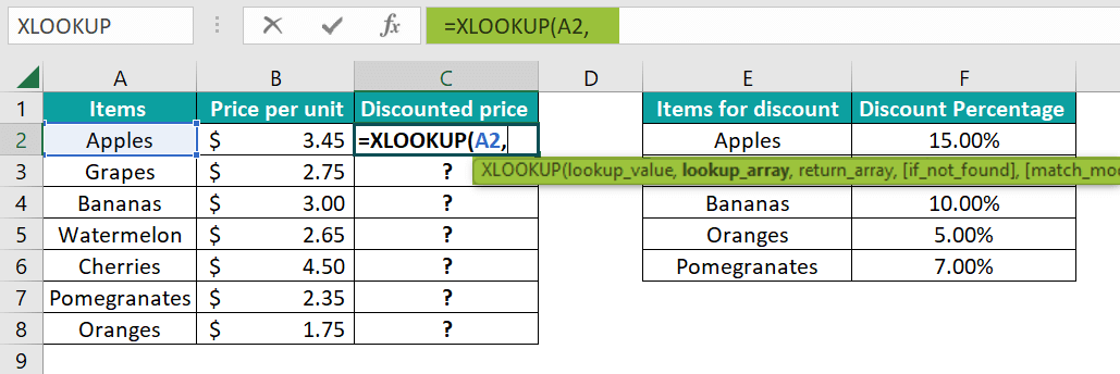

Step 2: Now, in this step, we can see that the respective Column E usually contains the item names, as well as Column F, the discount percentage effectively. And just after that, we just need to select the cells ranging from E2 to E6 and F2 to F6 as the lookup_array and return_array, respectively. Here, we will be adding the "$" to these two arrays to make them absolute references as well.

Step 3: Now, we are required to have the discounted price in Column C.

• For this, we will be multiplying the output of the function by the price per unit in cell B2.
• After that, we need to subtract it from the initial price B2 in order to get the discounted price.

Now, just after that, we need to apply the above changes; we enter the formula in cell C2 as

Now, we need to drag the Autofill handle from the cell ranging from C2 to C8 to get the discounted prices of each item.

Step 4: We must have noticed the #N/A error. More often, it primarily appears for items that do not have a discount specified in Columns E and F. To avoid this error, we need to supply the fourth argument to the formula as 0, respectively.

Step 5: Now, from the above step, we just need to press the Enter key from our keyboard. Drag the Autofill handle from C2 to C8 to get the discounted price of each item. Also, since we need to supply zero as the fourth argument, the items not found on the discount list have the same price after the discount.

INDEX MATCH Function in Microsoft Excel

It was well known, that the respective INDEX MATCH is an Excel function that usually combines out the INDEX as well as the MATCH formulas to allow users for the purpose of retrieving out the value in the advanced lookups as well. The former fetches out the value in the given table depending upon the column as well as the number of rows. In contrast, the latter returns the relative position of a value in a row or column, respectively. Moreover, it can look up values from left to right and right to left across a range of cells. As a result, it is considered the more suitable alternative for the VLOOKUP function.

Moreover, for instance, we can make use of the INDEX MATCH function in Microsoft Excel in order to find an employee's name that is based on their employee ID by making use of the data mentioned_ below:

First of all, we will be creating a reference of the cell, i.e., cell D2, containing the ID of the Employee (11 in this case as well). Next, we will try to fetch the name of the employee in cell E2 by just entering the formula as well:

The INDEX function looks for the employee's name in cells ranging from cell B2 to cell B10 based on the number of rows provided in the MATCH function for the employee ID 11 in cell D2 as well. The function returns the result as 'RAM,' which is the name of the employee with the ID 11 in the table array in an effective manner.

Syntax - INDEX + MATCH Function

We all know that the respective INDEX MATCH is usually a combo of the INDEX as well as the MATCH formula. Therefore, we can make use of it to get the desired result for the lookup value respectively.

So let us now understand the syntax of these two functions one by one in an efficient manner:

#1 - INDEX Function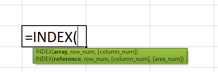

• Reference: It can be considered as the single cell range or the collection of the non-adjacent cell ranges, respectively.
• Row_Number: The first argument from the Array, from which we are required to fetch the value of the exact row number as well.
• [Column Num]: This is termed to be an optional argument from the Array, which we can use to fetch the value from the specified row as the column effectively.
• [Area_Num]: Again, this is an optional argument, which we can make use of for the multiple ranges for an argument. We can also provide the area number by just selecting the reference from all the available ranges efficiently.

#2 - MATCH Function

The respective MATCH function has mainly three arguments. Below is the image of the same: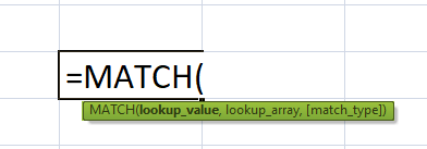

• Lookup_Value: The value whose position we want to locate in the lookup array (second argument), and it is a mandatory argument as well.
• Lookup_Array: More often, this will be either the range or the table array where we actually search for the lookup value, and it is also considered as the mandatory argument.
• [Match_type]: It is an optional argument and the matching criteria that we must define for the lookup value. It can be:

1 = It will mainly look for the largest value, either less than or equal to the lookup_value that we have provided, and return the approximate match. It will also require lookup_array to be arranged in ascending order (lower to higher or A to Z), respectively.

0 = It will look for and return the exact match to the lookup_value, irrespective of how the data is arranged or sorted.

-1 = This will search for the smallest value, either greater than or equal to the lookup_value you have provided, and return the approximate match. It requires the lookup_array to be arranged in descending order (higher to lower or Z to A).

How to make use of the Index + Match Excel Function?

The respective INDEX function usually searches for the value within the Array, which is based upon the row as well as the column number provided as well:

• For example, Below is the sales data for the different U.S. states in the different years as well:

And now, we will be finding out the sales value for the state NH for the year 2018.

Below are the steps to get the results respectively:

Step 1: First of all, we will be entering the INDEX function in the cell K3 as well.

Step 2: We are required to select the table array for the array argument, i.e., ranging from cell B2:I10.

Step 3: Now, we will be entering the row number from the Array to fetch the cell value. Here, we are trying to find out the value for the state NH; hence, the row number will be 4 (5th row in Excel).

Step 4: We are also looking for the value for a particular year as well. So, we are required to provide the column number for the table array. Here, we are trying to find out the value for the year 2018, and the column number will be 4 as well.

This finishes the INDEX formula. Now, close the bracket and hit the enter key to get the result, i.e., 4523 for NH.

We have manually provided the row as well as the column numbers to the Index Formula in the above steps. More often, it was well known that the respective MATCH function fetches out the position of a value in a row or the column that has been provided. First of all, we will be finding the number of row numbers for the state NH by just making use of the MATCH function.

Step 1: First of all, we are required to enter the MATCH function in the cell K4.

Step 2: And then the lookup value for the MATCH function would be "NH" in this case.

Step 3: Now in this step, we will be selecting out the range of the cells from A2:A10 for the lookup array in an effective manner.

Step 4: The last part is the match type. For this, we will be choosing 0 because we are looking for the exact match as well.

The function primarily returns the number of rows for the state NH as 4. Similarly, we can do the same in order to fetch the column number for any year, like as 2018.

The function will then return the column number for 2018 as 4, respectively.

We can now combine the MATCH function with the help of the INDEX function in order to get the row number as well as the column number dynamically. So, let us now find out the sales value for the state VB and the year 2021. Then, we will be entering the state name VB in cell K7 and the year 2021 in cell L6, respectively.

Next, we will use the MATCH and INDEX functions to automatically get the row and column numbers for the state VB and 2021.

Examples

Let us now look at some of the advanced examples of using the INDEX MATCH function in Microsoft Excel:

Example #1: An Alternative to VLOOKUP Function.

Now it is well known that the VLOOKUP is an advanced lookup function, and it has its limitations. Therefore, we can make use of the INDEX and the MATCH functions as an alternative to the VLOOKUP function in Microsoft Excel.

• For example, Below in the table, we have considered the age data for family members as well:

In this, we will be trying to find the age for the "Peter John" by just making use of the cell reference D2. Here, the lookup value (age) is to the right of the Array, and VLOOKUP cannot fetch the data from right to left.

Hence, we have to make use of the INDEX MATCH function to overcome the limitation of VLOOKUP in this scenario.

Step 1: First of all, we are required to enter the INDEX function in cell E2 as well.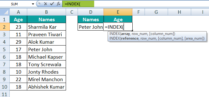

Step 2: Now, after that, we are required to select the age column array for the argument Array, i.e., A2:A10.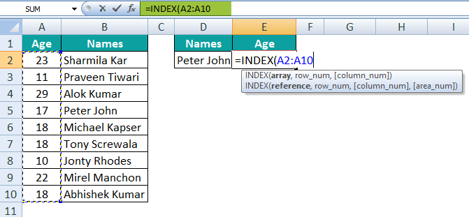

Step 3: Now, in this step, we just need to enter the Row Number argument in the MATCH function respectively.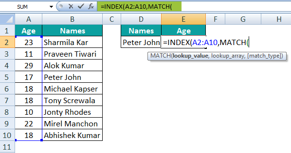

Step 4: And for the lookup value, we must need to select cell D2.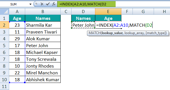

Step 5: And for the lookup array, we must need to select the range of cells, i.e., B2:B10.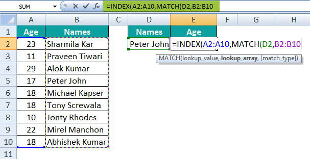

Step 6: The last argument is to select the match type. For this, we will choose the exact match, i.e., 0.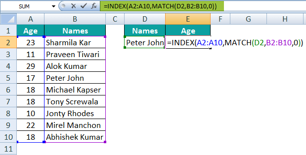

Step 7: Close the bracket. It will dynamically return the result as 17, which is the age of Peter John.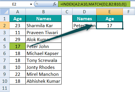

Thus, we can effectively make use of the MATCH formula as the supportive function for the INDEX formula as an alternative to the VLOOKUP function.

What are the key differences between the XLookup and Index match functions?

The primary key differences between the XLookup and the Index Match function are as follows:

1. Syntax:

• `XLOOKUP` has a simpler syntax, and it is mainly designed to be more user-friendly as well.
• `INDEX-MATCH` will effectively involve the use of the two separate functions, `INDEX` as well as the `MATCH,` which may be seen as less straightforward, respectively.

2. Direction:

• `XLOOKUP` will efficiently allow us to look up for the values both vertically and in horizontal manner with a single function, respectively.
• `INDEX-MATCH` typically requires the combination of both `INDEX` as well as the `MATCH` functions for the vertical lookups and more often it required an additional set up for the horizontal lookups as well.

3. Default Behavior:

• `XLOOKUP` has a default behavior for the approximate matches and it was quite similar to the `VLOOKUP' that we need to specify if we actually want an exact match explicitly.
• `INDEX-MATCH` allows more control over matching types, and thus offering flexibility in choosing between the exact, approximate, or the wildcard matches respectively.

4. Handling Errors:

• `XLOOKUP` has built-in error handling. If a match is not found, and it returns an error, but we can specify a default value or the custom error message.
• `INDEX-MATCH` may require the additional functions such as `IFERROR` to handle errors in an effective manner.

5. Array Handling:

• `XLOOKUP` can handle arrays natively, thus making it easier to work with the range of the data.
• And more often the respective `INDEX-MATCH` might require an array formulas for the purpose of handling array.

6. Compatibility:

• And it was well known that the `XLOOKUP` function is available in Microsoft Excel 365 and also in the version 2019 but it may not be available in the older versions as well.
• `INDEX-MATCH` is basically a combination of the functions which are made available in a broader range of the Microsoft Excel versions.

It could be concluded that the respective `XLOOKUP` function is more straightforward, user-friendly, and has built-in error handling, and in contrary to this the `INDEX-MATCH` offers more flexibility and is compatible with a wider range of the Microsoft Excel versions, thus making it a preferred choice for the certain scenarios.