Countif Function in Excel

One of the well-known functions in Excel is called Countif. The countif function in Excel is used to count the numbers, texts, and dates present in the cell. It meets the given condition called criteria. Countif function meets single criteria.

Syntax

COUNTIF (range, criteria)

Parameters

The two arguments are,

Range - The range is defined as the range of cells where the specified condition is applied

Criteria - The criteria mention the required condition where logical operators are included if necessary.

What are the criteria applied in the COUNTIF function?

The criteria include logical operators and wildcards. The logical operators include (>, <,>=, <=, <>). The wildcards include (.*,?), used in partial matching.

Examples of the COUNTIF function

Here are some examples of COUNTIF functions using logical operators and wildcards.

Example 1: Display the count of a number greater than 75 from the given data using the COUNTIF function.

Step 1: Enter the data in the required cell, namely A1:A10

Step 2: Here, in this example, to display the data greater than 75, the logical operator used is '>', called greater than a symbol. Select a new cell and enter the formula as =COUNTIF (A1:A10,">75")

Step 3: Press Enter. The result will display in the selected cell, which is the count of numbers greater than 75.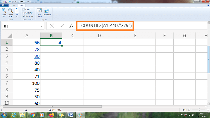

The above worksheet will display the result as 4, the count of a value greater than four.

Example 2: Display the count of a number equal to 50 from the given data using the COUNTIF function.

1. Enter the data in the required cell, namely A1:A10
2. Here, in this example, to display the data equal to 50, type the required number within the apostrophe or as it is. Select a new cell and enter the formula as =COUNTIFS (A1:A10,"50") or =COUNTIF (A1:A10, 50)
3. Press Enter. The result will display in the selected cell, which is the count of numbers equal to 50.

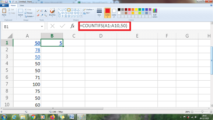
The above worksheet will display the result as 5, the count of values equal to 50.

Example 3: Display the count of a number less than or equal to 50 from the given data using the COUNTIF function.

1. Enter the data in the required cell, namely A1:A10
2. Here, in this example, to display the data which is lesser than or equal to 50, use the logical operator '<=' called lesser than or equal to. Select a new cell and enter the formula as =COUNTIF (A1:A10,"<=50").
3. Hit the Enter. The result will display in the selected cell, which is the count of numbers that is lesser than or equal to 50.

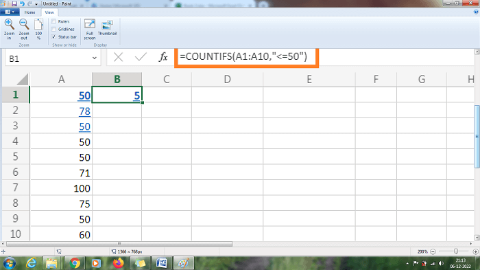
The above worksheet will display the result as 5, the count of numbers lesser than or equal to 50. In example 3, the formula's number is enclosed with the curly braces and the logical operator. In example 2, the required number is entered in the formula without double quotes. But if a logical operator is included with the double number quote ("") is used.

Example 4: Display the count of the number equal to the color green from the given data using the COUNTIF function.

1. Enter the data in the required cell, namely A1:A10
2. Here, in this example, to display the data equal to the color green, type the color name as it is in the formula. Select a new cell and enter the formula as =COUNTIF (A1:A10, "green").
3. Press Enter. The result will display in the selected cell, which is the count of numbers equal to green.

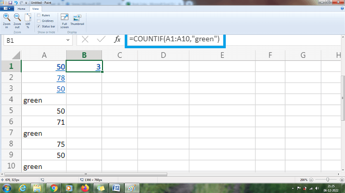
The above worksheet will display the result as 3, with the count of values equal to green.

Example 5: Display the count of numbers not equal to the color green from the given data using the COUNTIF function.

1. Enter the data in the required cell, namely A1:A10
2. Here in this example, to display the data not equal to the color green, use the logical operator '<>' called not equal to. Select a new cell and enter the formula as
   =COUNTIF (A1:A10,"<>green").
3. Press Enter. The result will display in the selected cell, which is the count of numbers that is not equal to green.

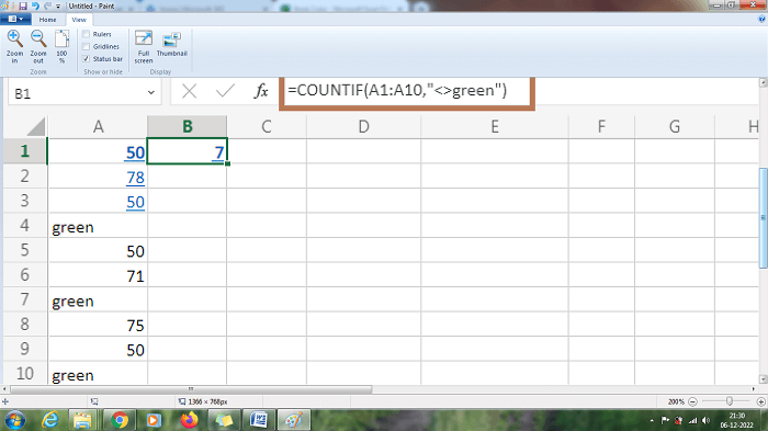
The above worksheet will display the result as 7, the count of values not equal to green.

Example 6: How to count blank cells in the given data using the COUNTIF function?

1. Enter the data in the required cell, namely A1:A10
2. Here, in this example, to display the blank cell, use "called double quote. Select a new cell and enter the formula as =COUNTIF (A1:A10,").
3. Press Enter. The result will display in the selected cell, which is the count of the number of blank cells in the data.

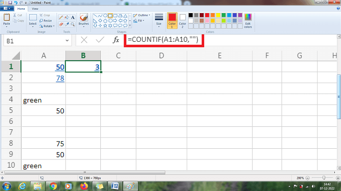
The above worksheet shows cells A3, A6 and A7 are blank cells. Hence the result will be displayed as 3, which is the count of blank cells in the given data.

Example 7: How to count non-blank cells in the given data using the COUNTIF function?

1. Enter the data in the required cell, namely A1:A10
2. Here in this example, to display the non-blank cell, use the logical operator <> called not equal to within double quotes"<>". Select a new cell and enter the formula as =COUNTIF (A1:A10,"<>").
3. Press Enter. The result will display in the selected cell, which is the count of the number of non-blank cells in the data.

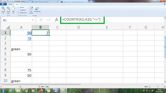
From the above worksheet the cell name A1, A2, A4, A5, A8, A9, and A10 are non-blank cells. Hence the result will be displayed as 7, which is the count of non-blank cells in the given data.

Example 8: How to count cells starting with particular alphabets using a formula?

1. Enter the data in the required cell, namely A1:A10
2. In this example, type the alphabet along with the asterisk symbol to display the cell starting with particular alphabets. Select a new cell and enter the formula as =COUNTIF (A1:A10," a*").
3. Press Enter. The result will display in the selected cell starting with alphabet A.

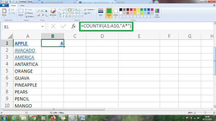
From the above worksheet, the data starting with the alphabet 'A' are Avocado, Apple, America, and Antarctica. Hence the result will be displayed as 4 which is the data count starting with the letter A.

Example 9: How to compare two cells using the formula?

1. Enter the data in the required cell, namely A1:A10
2. Here, in this example, to compare the data in two cells, type the respective cell name along with the logical operator > or < (greater than or lesser than). Select a new cell and enter the formula as =COUNTIF (A1:A10,"<"&A1).
3. The result will be displayed in the selected cell, which is the comparison of multiple cells

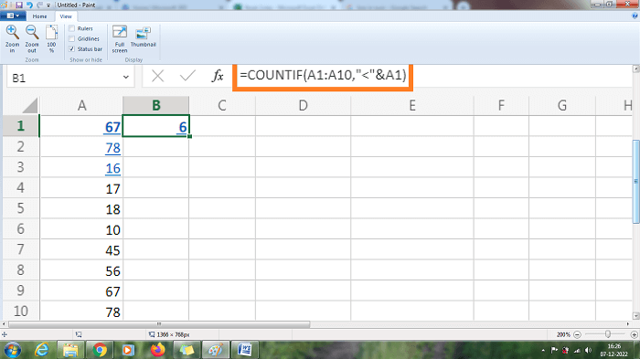
The above worksheet compares the value present in cell A1 with cell A2:A10. The result will be displayed as 6, the count of numbers lesser than the value in cell A1.

Example 10: How to compare the dates present in the cells using the formula?

1. Enter the data in the required cell namely A1:A10
2. Here in this example to compare the dates present in the cells, type the logical operator > or < (greater than or lesser than) along with the TODAY () function. Select a new cell and enter the formula as =COUNTIF (A1:A10,"<"&TODAY ()).
3. The result will be displayed in the selected cell, which is the comparison of multiple cells

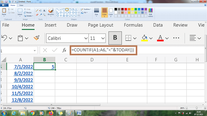
From the above worksheet, the result will be displayed as 5 which is the count of numbers lesser than the present date. The date present in cell A6 is greater than the present date. Hence the formula counts the rest of the cells using concatenation with the character ampersand (&).

In example 9 and example 10 the concatenation concept is used. Here the COUNTIF function retrieves the value and then concatenates with the logical operator present in the formula.

Example 11: Is case sensitive applicable to the COUNTIF function?

Step 1: Enter the data in the required cell, namely A1:A10

Step 2: Here, in this example, to check the case-sensitive, type the required arguments in the formula. Select a new cell and enter the formula as =COUNTIF (A1:A10,"orange")

Step 3: The result will be displayed in the selected cell, the count of oranges in the given data.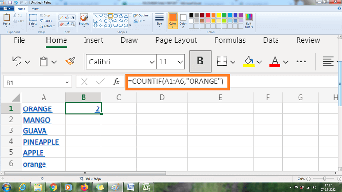

The above worksheet will display the result as 2 which is the count of oranges. In cells A1 and A6, the data "orange "is present in both upper and lower case. The formula counts upper and lower-case data and displays the result. Hence COUNTIF function is not case-sensitive.

Example 12: How to compare the data in the cell with the user-specified date?

In example 10, the present date is compared with the data present in the cell. But what is the solution if the user wants to compare the data with their specified or desired date? To solve this query, the steps to be followed are,

1. Enter the data in the required cell, namely A1:A10
2. In this example, to check the data with a specified date, type the required or specified date in the formula. Select a new cell and enter the formula as =COUNTIF (A1:A10,"<"& DATE (2022, 6, 7)). Here the date entered is 7 th June 2022.

Step 3: The result will be displayed in the selected cell, the count of data lesser than 7^th June 2022.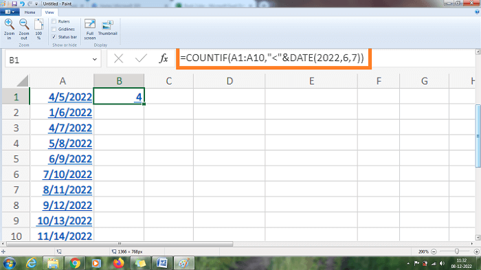

The above worksheet will display the result as 4, the count of dates lesser than 7^th June 2022. Similarly, by modifying the formula, the user can enter the required date in the formula method.

Examples 1 and 12 explain the COUNTIF function using logical operators. Next, let's have a look at wildcards. As previously mentioned, wildcards include the symbols of the question mark (?), the asterisk (*), and the tilde.

Example 12: How to count the specified data present in the cell?

Sometimes the single cell contains lengthy data, where counting only the specified word is a tough process. To count the particular word in the lengthy data, the wildcard symbol asterisk (*) is used. The steps to be followed are,

Step 1: Enter the data in the required cell range A1:A5

Step 2: In this example, to check how often the specified word is repeated, type the respective word along with the asterisk symbol(*). Select a new cell and enter the formula as =COUNTIF (A1:A10,"*orange*")

Step 3: The result will be displayed in the selected cell, the count of oranges present in the given data.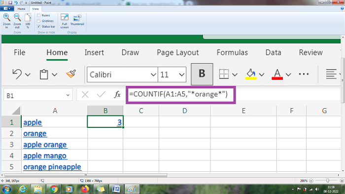

From the above worksheet, the result will be displayed as 3 which is the count of the word "orange" present in the given data, even though orange is combined with other fruit.

What happens if the data is typed in the formula without an asterisk?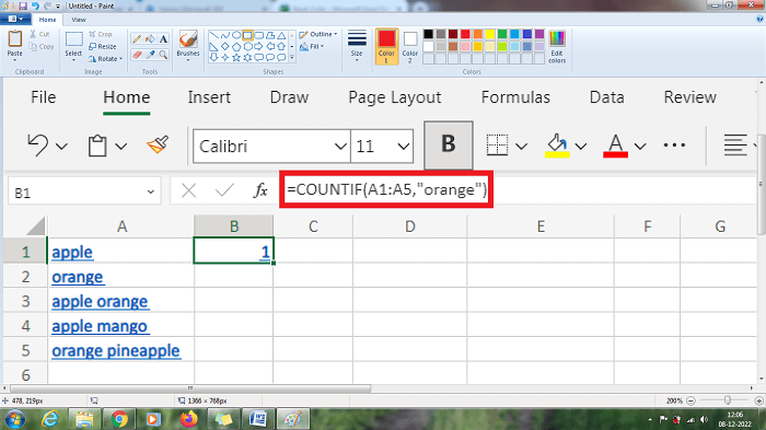

The above worksheet shows the result as 1 as the COUNTIF function counts the word "orange," which is present separately in the cell.

What happens if the data is typed in the formula starting with an asterisk but not in the ending?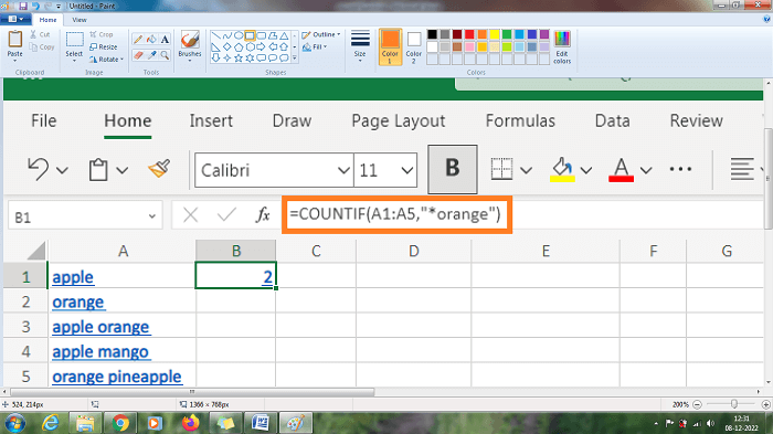

The above worksheet shows the result as 2, which is the data count starting with the word orange. In cell A3 the data "apple orange" is not counted as orange is present in the last. If an asterisk is present only at the start of the data, it counts only the data starting with the specified word.

Example 12.2: How to count the number of characters present in the data using the COUNTIF function?

To display the specified amount of characters present in the data, the steps to be followed are,

Step 1: Enter the data in the required cell range A1:A5

Step 2: To display the specified word count data, use the wildcard symbol question mark (?). A single question mark implies a single character. Select a new cell and enter the formula as =COUNTIF (A1:A10,"????"). Here the data with 5 characters are counted

Step 3: The result will be displayed in the selected cell, the count of five-letter data present in the given data.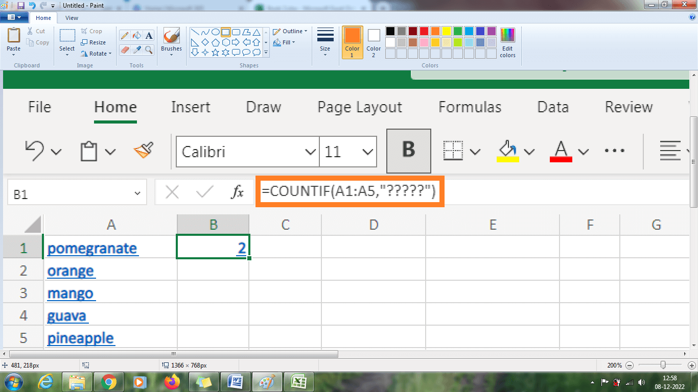

From the above worksheet, the result is displayed as two (orange, mango), the count of data present with five characters.

Example 12.3: How to apply more than one condition in the Countif function?

By default, the Countif function is designed to accept one condition. But to count cells that have multiple data, the array constant and SUM function is used. The steps to be followed are,

Step 1: Enter the data in the required cell range A1:A5

Step 2: Here, in this example, to display the count of specified data, use the array constant in the formula. Select a new cell and enter the formula as =SUM (COUNTIF (A1:A5, {"apple","mango"}))

Step 3: The result will be displayed in the selected cell which is the count of apples or mango present in cell A1:A5.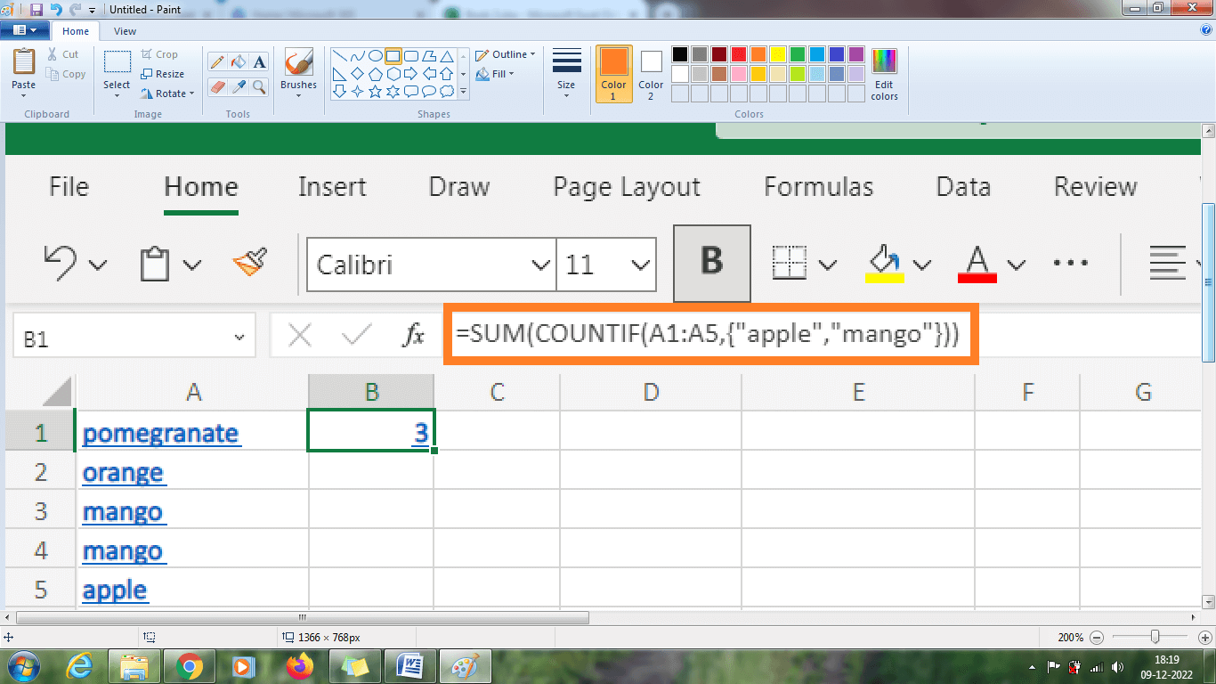

The above worksheet will display the result as 3, the count of apples or oranges present in cell A1:A5.

Summary

The above tutorial explains the various methods to count the data using the COUNTIF function. It is used to count the data effectively and quickly.