How to Unfreeze Excel on mac

Freezing the cells in MS Excel on mac OS

MS Excel allows the user to freeze the cells that contain such data that the user does not want to format or change.

It allows you to freeze and unfreeze cells both vertically and horizontally. The user can also freeze or unfreeze an entire row or column in your spreadsheet.

When the user freezes the entire column or row in the spreadsheet, then no changes can be implemented in the cells of that row or column. The cells that the user freezes are always displayed on the screen until the user works on the spreadsheet. If the user opens the spreadsheet, the frozen cells are displayed.

Freezing and Unfreezing the panes to lock a column or row in MS Excel

In mac OS

Imagine a situation where you want to scroll down the data in the spreadsheet, but at the same time, you want to refer to the data. This can be easily done by freezing those particular cells. After freezing the data, it will be displayed on the screen even when the user is scrolling the data.

Implementing Freeze in the Cell

1. The user can freeze the spreadsheet cells directly by using the Freeze button in the View tab.
2. If the user does not see the freeze buttons in the View tab of the application, then the user needs to ensure that the user switches to the Normal View.
3. To open the Normal View, from the View tab. Click on Normal.
4. Now the Freeze button will appear in the View tab.

Freezing the Top Row in mac OS

1. Open the spreadsheet in your MS Excel application.
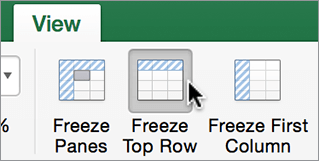
2. Switch the Home tab to the View tab. In the view tab, click on the Freeze top Row.
   
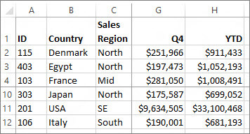
3. After selecting the Freeze Row option, the first row of the spreadsheet will be frozen. The user can ensure that the row is frozen.
4. A border will appear just below the first row of the spreadsheet. The border is darker than the border below the other rows of the spreadsheet.

Freezing the First column in mac OS

1. Open the spreadsheet in your MS Excel application.
2. Switch the Home tab to the View tab. In the view tab, click on the Freeze first column.
   
3. After selecting the Freeze First Column option, the first column of the spreadsheet will be frozen. The user can ensure that the column is frozen.
4. A border will appear just to the left of the frozen column of the spreadsheet. The border is darker than the border below the other rows of the spreadsheet.

Freezing the top row and the first column Simultaneously

In MS Excel, the user can simultaneously freeze the top row and the first column of the spreadsheet.

1. To do so, select the B2 cell in the spreadsheet.
2. After selecting the cell, click on the View tab. From the menu, click on Freeze Pane.

Freezing Multiple Rows and Columns in MS Excel in mac OS

In MS Excel, the user can freeze multiple rows and columns. This is only possible if the user begins freezing the rows and columns from the first row and column.

Let us freeze the multiple rows and columns in the spreadsheet:

1. The user needs to begin with the sheet's first row and then continue to select the last row just below the last row that you want to freeze.
2. Once you have selected both rows, click on the Freeze Panes in the View tab.
3. Let us discuss this using an example if the user wants to freeze the first four rows of the spreadsheet and the three columns from the left of the spreadsheet.
4. The first step is to click on the cell just below the last joint of the pane. In this case, it is D5 to determine the cell. It should be just below the row to be selected and right to the cell's column.
5. Once selecting the cell, click on the Freeze Panes in the View tab. The border below the row and right to the column will appear a little thicker than the other border.

Unfreezing the Rows and Columns in the mac OS

If the user wants to unfreeze the spreadsheet row or column, follow the given steps.

1. First, he/she has to select the frozen row or column.
2. Then, he can click on the Unfreeze Panes from the View Tab.