| |

How to Split Cells in ExcelMS Excel or Microsoft is the popular spreadsheet program that most people use for different tasks. Sometimes, we may get the wrongly formatted data while downloading it from the web or getting it extracted from other software. The typical case is when we have different data in the same cell that must be broken up into different cells. The data may be separated by a comma, semicolon, tab, or any other character. In such situations, we need to split the cells in Excel. For example, we might have full names of people in a single cell, and we may need to split these into first names and the last names in consecutive columns. In this article, we are discussing three simple methods that help us to split cells in Excel, such as:
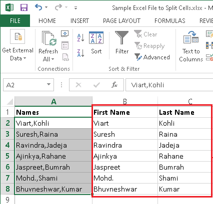
In all of the above methods, we will use the following data set as an example, where we have a single cell with two different items (First Name, Last Name) separated by a comma: 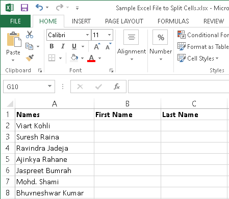
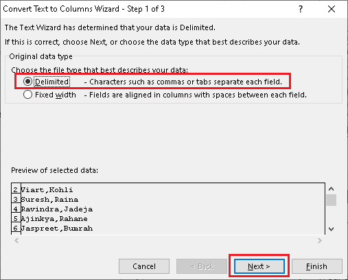
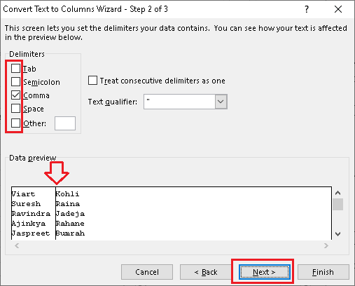
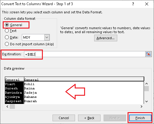
Let us discuss each method in detail: Split Cells in Excel Using Text to ColumnsOne of the simplest and commonly used methods to split cells in Excel includes using the Text to Columns tool. This method allows us to split the whole columns with all cells using the desired rules of separating the data. The tool can easily separate the data of the cells, whether the separating text is a comma, space, tab, etc. Although this particular method is the best way to split cells in Excel, we need to try other ways to split hundreds or thousands of cells. Depending on the data, one method may produce better results than others. The lower the level of data consistency, the more difficult the process becomes. The method of splitting a cell using the Text to Columns tool are as follows:
Split Cells in Excel Using Flash FillThe flash fill feature is another handy way of splitting cells in Excel. However, this feature is only available in Excel 2013 and above. The flash fill method works by self-identifying the patterns and then applying corresponding patterns for all the consecutive cells. This method only works when we need to split the data into the connected cells. Flash fill typically works in two ways:
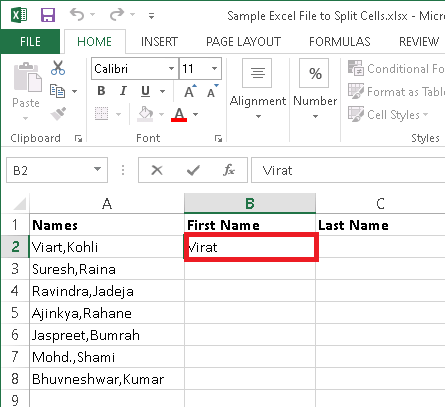
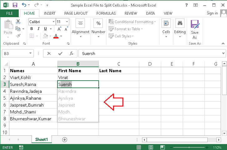
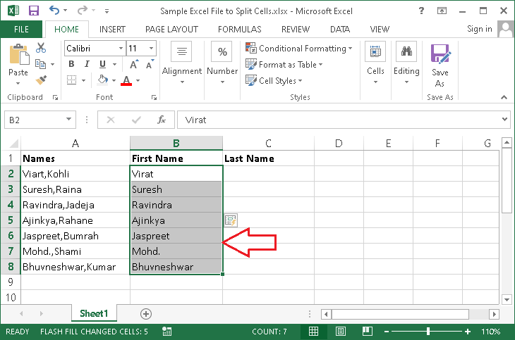
Background Execution by ExcelExcel automatically tries to find certain patterns in the background and then suggests users make the changes accordingly. Let us understand this with an example:
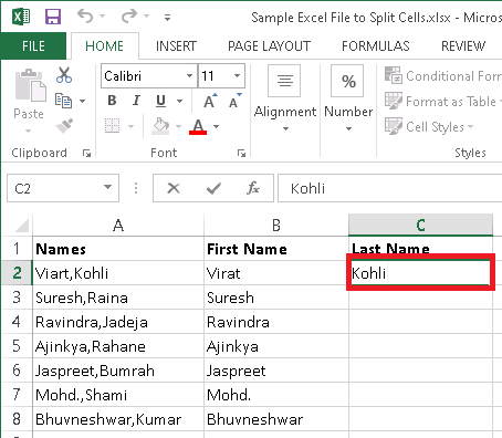
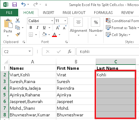
Manually Triggered wherever neededIf Excel does not provide recommendations to split the data, we can manually trigger Flash fill in Excel. Let us now extract the last names using manual execution:
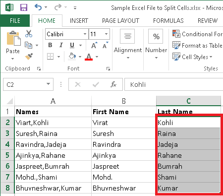
That is how we can split the cells in Excel using the Flash fill. We can try any of the Flash fill methods, such as the background or manual methods. Split Cells in Excel Using Text FunctionsThe last and most efficient method to split cells in Excel includes the use of specific functions. This method is dynamic and works with any data. Although this method allows us to split data with certain rules applied to programs, we must have some advanced Excel skills. While the method is powerful, it is not just a point-and-click method. Instead, we need to efficiently think and apply proper functions with proper rules to split cells accordingly. The following are the useful functions required for splitting Excel cells in many cases: LEFTThis function returns the specified number of characters set from the beginning of the selected text string/ cell(s). For example, suppose we use this function as: We will get the result as: WELC Argument (4) tells the function only to return the initial four characters of the text string "WELCOME USER". RIGHTThis function returns the specified number of characters set from the selected text string/ cell(s) endpoint. For example, suppose we use this function as: We will get the result as: USER Argument (4) tells the function only to return the last four characters of the text string "WELCOME USER". MIDThis function returns the specified number of characters from the middle of the selected text string/ cell(s). However, the starting position and length must be defined. For example, suppose we use this function as: We will get the result as: COME The second argument (initial 4) gives the function the nth character to start from, and the last argument (last 4) defines the length of the output string. Thus, the four characters starting at position four are "COME" in the string "WELCOME USER". LENThis function only returns the total number of characters available in a selected text string/ cell(s). For example, suppose we use this function as: We will get the result as: 12 It is because the string "WELCOME USER" has a total of 12 characters, including space. SEARCHThis function typically returns the total number of characters at which the specified character or text string is first found. The function reads the given string from the left character to the right and is not case-sensitive. For example, suppose we use this function as: We will get the result as: 8 The specified character (space) is initially located at the 8th position of the given string "WELCOME USER". The last argument (1) is optional and is mainly used to tell the function where to start searching the specified character. Similarly, the FIND function is also used, but it is case-sensitive, unlike the SEARCH function. SUBSTITUTEThis function typically replaces the specified characters with the newly defined characters in the selected text string/ cell(s). For example, suppose we use this function as: We will get the result as: WELCOME DEAR The last specified argument (1) defines which instance to replace. In the above example, only one instance exists, which is also the first instance. It is because the text characters "USE" are replaced with "DEA". If we needed to replace more, we could change the number of arguments accordingly. Let us now apply the necessary functions and rules with our example data: We need to split the first names and the last names from the cells. For this, we need to use LEFT, RIGHT, SEARCH, and LEN functions in the following ways: First NameFor the first names, we use the following function: We will get the result as: 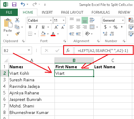
Where,
Last NameFor the last names, we use the following function: We will get the result as: 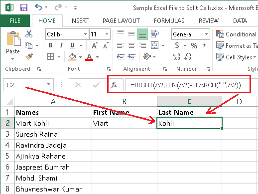
Where,
After applying both the above functions in all the individual cells, we get the following results: 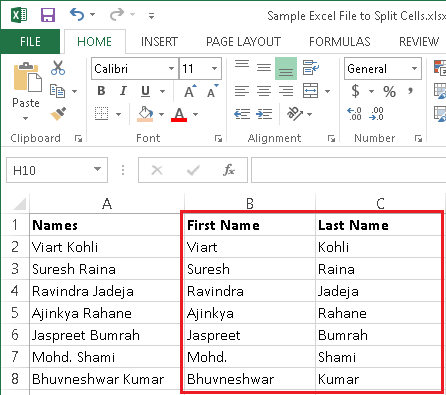
That is how we can split cells in Excel using the text functions.
Next TopicCurrent Date in Excel
|
 For Videos Join Our Youtube Channel: Join Now
Feedback
- Send your Feedback to [email protected]
Help Others, Please Share


