Excel TRIM Function

The Excel data is usually imported from different databases or other data applications. The data fetched from these sources are usually not in proper order. They contain leading, trailing, or irregular spaces, and these spaces affect the output of your formulas. For example, you compare the data of two different columns for duplicate values that you know are present there, but the Excel function cannot locate the duplicate data. Or, when you add up numbers from two columns but end up getting zero as your output. These are only some examples of problems generated by leading, trailing, or in-between spaces in the cells containing numeric or text values.

Though there are many methods to remove extra spaces and clean up your data in Microsoft Excel, but the easiest and fastest solution to delete the extra spaces is Excel's inbuilt TRIM function.

What is TRIM function?

The Excel TRIM function removes before and following spaces from the words, i.e., leading and trailing spaces. It also eliminates extra spaces in-between the texts but does not remove the single space separating two different texts. In other words, we can say that the TRIM function is used to clean the unwanted space characters from your data.

This function strips extra spaces from your numeric or text values, leaving only a single space between words and excluding any leading, trailing, or extra in-between space. Microsoft Excel designed the TRIM function to eliminate only the space character, which has value 32 in the 7-bit ASCII code system. Apart from extra spaces, sometimes our data contains line breaks and non-printing characters. In such cases, the TRIM function will only remove the extra spaces. If you intend to clean your data and remove the line breaks and various non-printing characters (7-bit ASCII code values 0 through 31) use the TRIM function in combination with the Excel CLEAN function.

Syntax

Parameter

Text (Required): This parameter represents the text from which you want to remove the extra space.

Points to Remember about the TRIM Function:

• The TRIM() function strips the extra spaces from the given text. Therefore, leaving only a single space between words and removing all the space characters at the start or end of the text and the extra spaces in between text.
• This function is useful to clean the unnecessary mess that you receive by importing your data from other applications or environments.
• Technically, TRIM only removes the character has value 32 in the 7-bit ASCII code system.
• Sometimes TRIM does not work and it may be because your text contains Unicode character also known as non-breaking space character (160) that is commonly used in web pages as the html character  . TRIM function cannot remove these nonbreaking spaces.
• If you want to remove unwanted elements you can use the Excel CLEAN function. It strips the first 32 non-printing characters (7-bit ASCII code values 0 through 31) from the given data.

Example 1: In the below table, Use TRIM to remove the extra spaces.

The TRIM function removes all leading, trailing and in-between spaces leaving a single space character in between the text. To trim you data follow the below given steps:

STEP 1: Add a helper column named Trimmed Output

Place your mouse cursor to the cell next to "string1" and name the new column as "Trimmed Output".

It will look similar to the below image: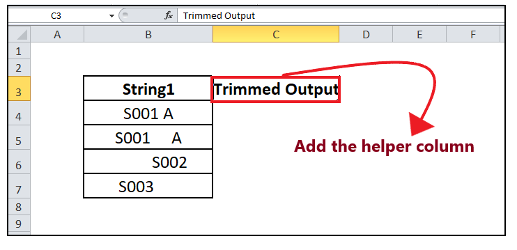

In this column we will type our TRIM formula and place the trimmed data for different text values.

NOTE: Format the helper column and match it with the first column to make your Excel sheet more attractive.

STEP 2: Type the TRIM formula

Put your cursor to the second row and start typing the function = TRIM(

It will look similar to the below image: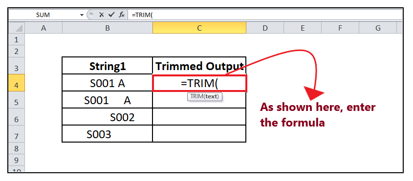

STEP 3: Insert the text parameter

The text parameter represents the input value from which you want to remove the extra spaces. Here, B4 represents the text cell.

It will look similar to the below image: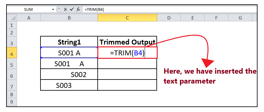

STEP 4: TRIM will return the result

The TRIM will return the data after removing the extra leading, trailing or in-between spaces leaving only a single space between words.

It will look similar to the below image: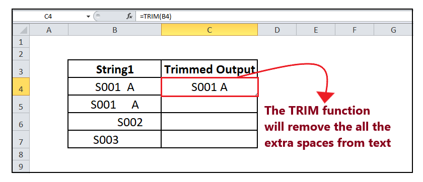

STEP 5: Drag the formula to other rows to repeat

Place your mouse cursor on the formula cell and point the cursor to the right corner of the cell. To your surprise, the mouse pointer will turn into a '+' icon.

Refer to the below image: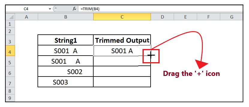

Drag the '+' icon down the cells. It will copy the TRIM function to all your cells changing the cell reference as respective to the cell. As you can see below, the extra spaces from your data has been removed.

It will look similar to the below image: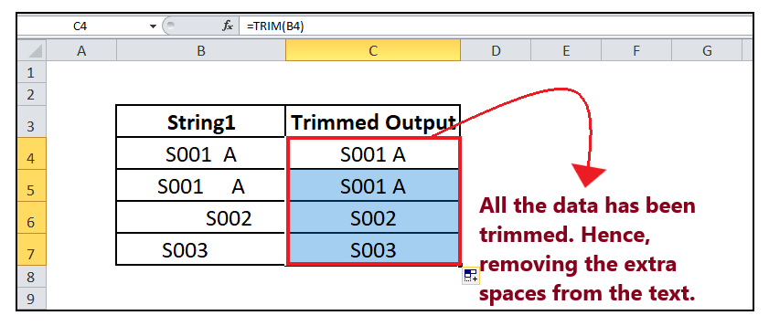

That's it; following the above few steps, you can easily remove the extra spaces from your text.

Example 2: Remove the extra spaces in the strings and then join the 3 strings together using CONCATENATE and & (ampersand) operator to get the results as mentioned in the result column. Do so in one formula itself

STEP 1: Add a helper column named Output

Place your mouse cursor to the cell next to "string1" and name the new column as "Output".

It will look similar to the below image: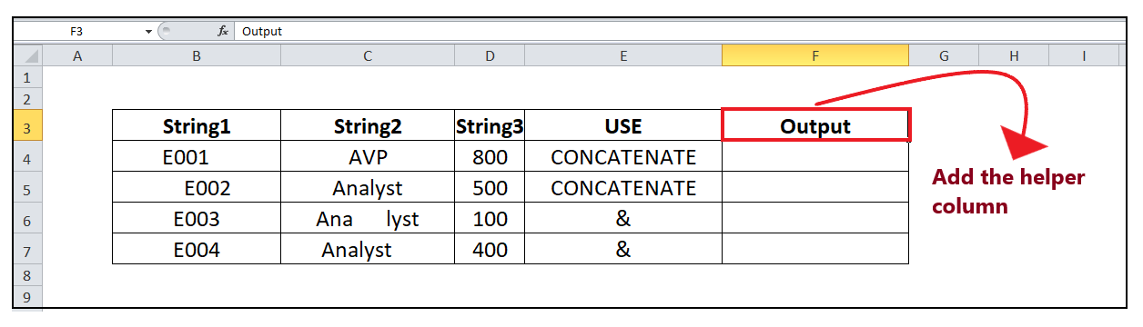

In this column we will type our TRIM formula and place the trimmed data for different text values.

NOTE: Format the helper column and match it with the match column to make your Excel sheet more attractive.

STEP 2: Type the TRIM formula

Put your cursor to the second row and start typing the function = TRIM(

It will look similar to the below image: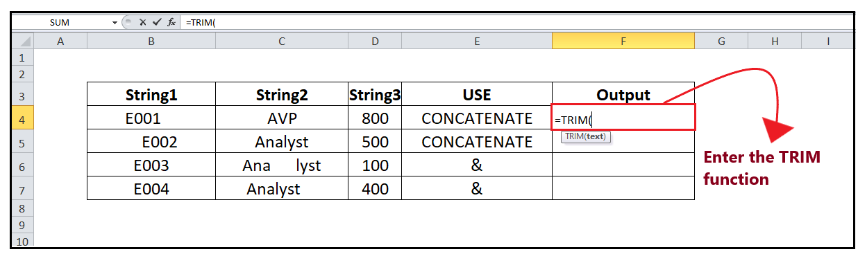

Next, we are supposed to concatenate the three strings, inserting the Excel CONCATENATE function inside the TRIM function.

Refer to the below image: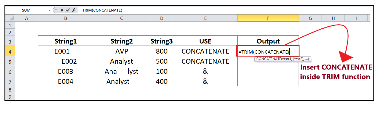

STEP 3: Add the parameter

Next, we will pass the strings. Firstly we will pass string1, and therefore here we have referred to cell B4. Separated by comma, we will pass the reference of the second cell, i.e., C4. Again we will separate it by comma and pass the reference of the third cell, i.e., D4.

The formula will become: =TRIM(CONCATENATE(B4,C4,D4))

It will look similar to the below image: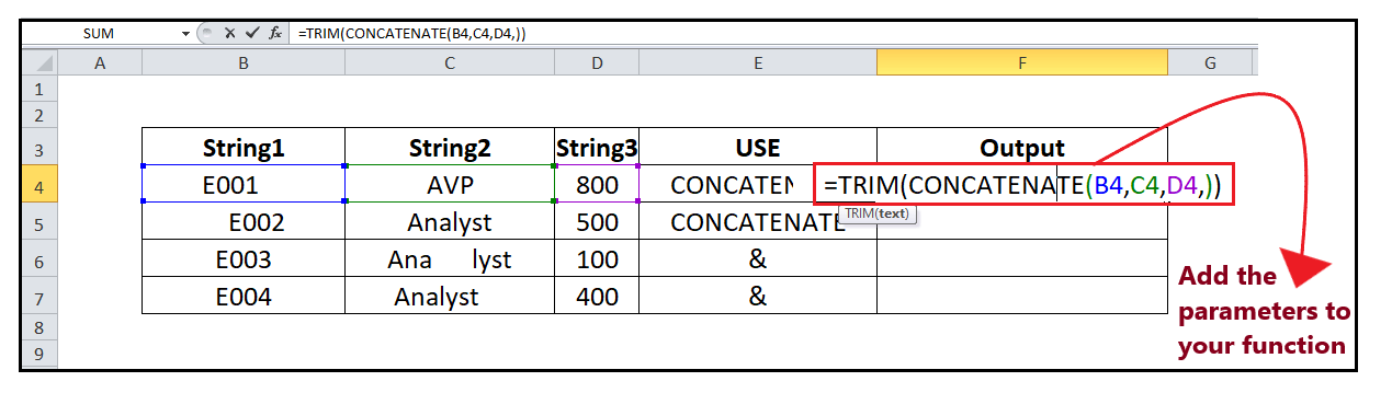

STEP 4: TRIM will return the result

The concatenate will add three of the strings, and afterward, the TRIM function will remove all the extra spaces from the text leaving only a single space between words.

It will look similar to the below image: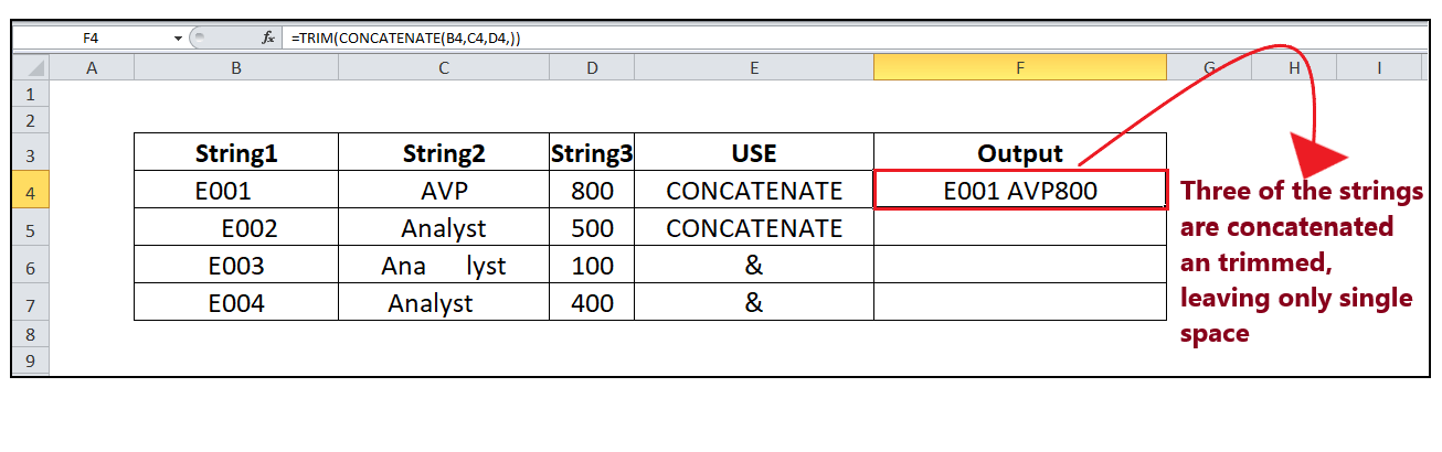

STEP 5: Drag the formula to next rows to repeat

Place your mouse cursor on the formula cell and point the cursor to the right corner of the cell. To your surprise, the mouse pointer will turn into a '+' icon. Drag the icon to repeat the formula for the next row.

Refer to the below image: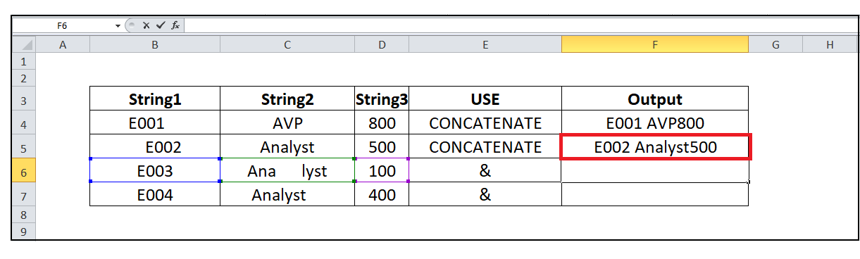

STEP 6: Insert the TRIM formula and use & to combine the strings

• Point your cursor to the next row and enter the formula = TRIM(
• Enter the parameter by referring to the first string followed by '&'. Next, refer to the second string followed by the '&' and again refer to the third-string cell.
• The formula will become: =TRIM(B6&C6&D6)

Refer to the below image: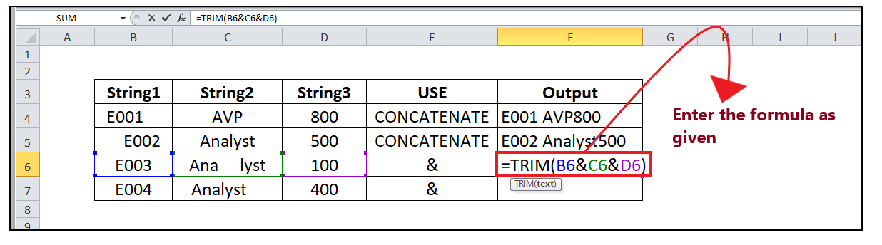

STEP 7: Drag the formula to F7 cell

Drag the '+' icon down the cells. It will copy the TRIM function to all your cells, changing the cell reference as respective to the cell.

As you can see below, the extra spaces from your text (including the leading, trailing, and extra in-between spaces) have been removed.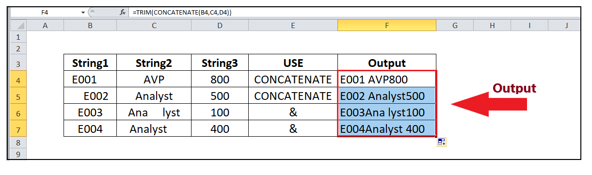

Example 3: Remove only leading spaces from Excel data (Left Trim)

In some cases, you may intentionally insert double or triple space characters in between your data values to make your text visually attractive and more readable. However, you do want to remove the unwanted leading spaces. To do so, follow the below-given steps:

STEP 1: Add a helper column named Output

Place your mouse cursor to the cell next to "string1" and name the new column as "Output".

It will look similar to the below image: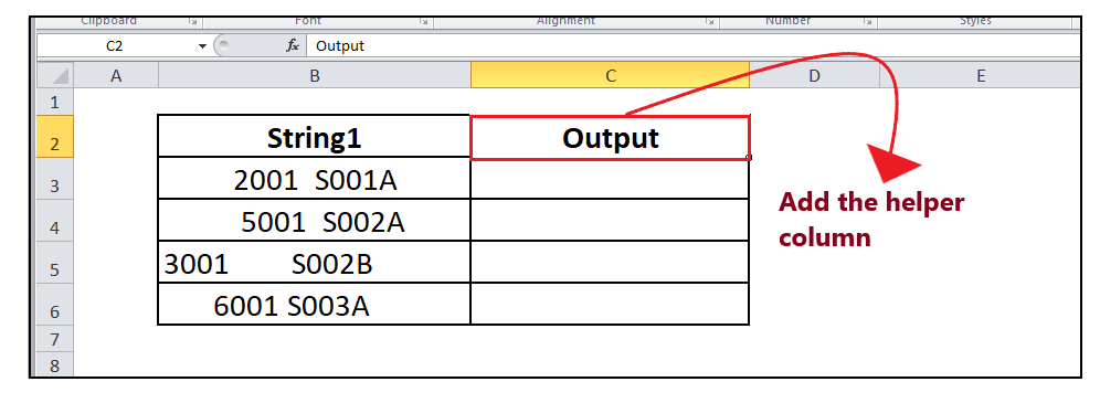

In this column we will type our formula and place the trimmed data for different text values.

STEP 2: Insert the formula

As you already know, the TRIM function also removes the unwanted spaces that are present in between the data values. But if you want to keep all the in-between white spaces intact, the TRIM function alone won't work; you have to construct a bit more complex formula:

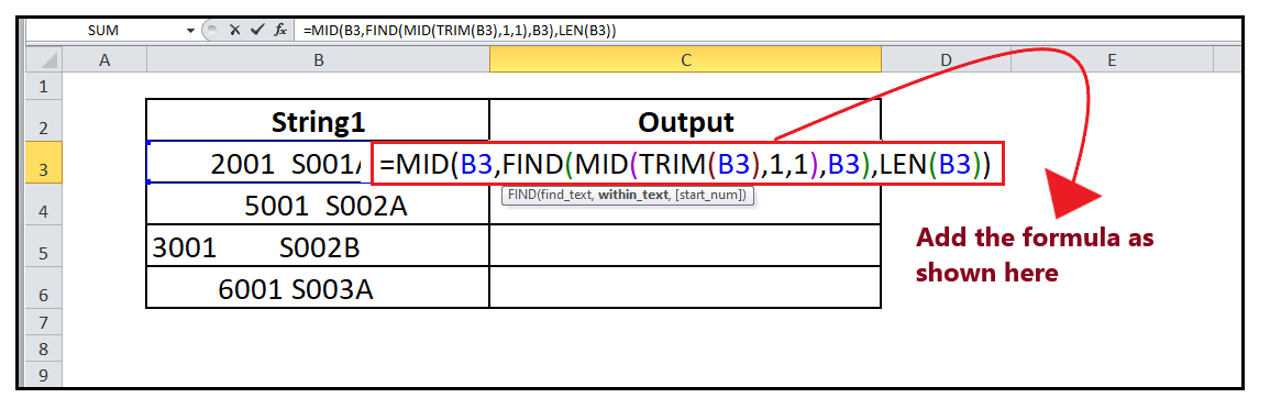
In the above formula, the grouping of FIND, MID, and TRIM locates the position of the first value of your string. And then, we have provided the fetched number to another MID function to return the entire text string (where the LEN function computes the string length) starting at the position of the first text character.

STEP 3: TRIM will return the result

The TRIM function will return the result after removing only the leading spaces from your text value.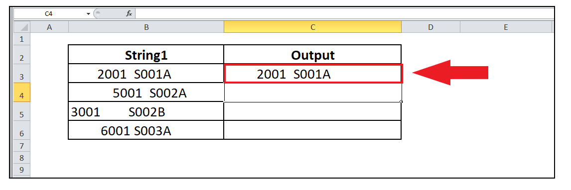

NOTE: Unlike here we have removed the leading spaces. Similarly, you can remove spaces from the end of cells, by modifying the formula a bit.

STEP 5: Drag the formula to other rows to repeat

• Place your mouse cursor on the formula cell and point the cursor to the right corner of the cell.
• To your surprise, the mouse pointer will turn into a '+' icon. Drag the '+' icon down the cells.
• It will copy the TRIM function to all your cells, changing the cell reference as respective to the cell.
• As you can see below, all the leading spaces from the data have been removed.

Refer to the below image: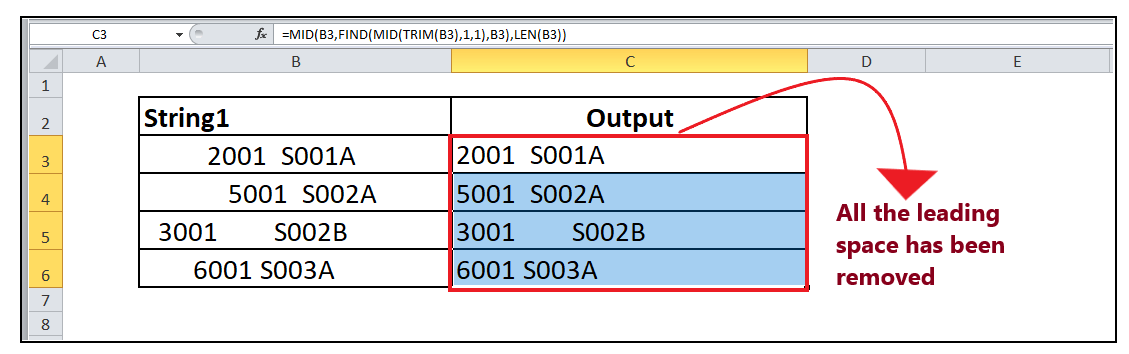

Excel TRIM not working

The TRIM function is designed only to remove the space character represented by code value 32 in the 7-bit ASCII character set. Sometimes you copy the Excel data from different websites and while pasting the data you paste some Unicode characters as well. In the Unicode character set, there is one more space character known as the non-breaking space (having a decimal value of 160), commonly used in web pages as the html character  . TRIM function cannot remove this Unicode space character.

So, if your Excel worksheet contains unwanted space character that the TRIM function cannot eliminate, don't get panic and use the Excel SUBSTITUTE function to convert the Unicode space character into regular Excel white spaces and then apply the TRIM function.

Let's suppose the text is present in B1, the formula will be as follows: