Excel Multiply Formulas

Multiplication

"Multiplication is one of the arithmetic operations used to find the total number of items or products in the given data." In other words, it is called the repeated addition of products of equal size. There are various symbols of multiplication which are represented as follows:

1. Signs cross(x)
2. Asterisk (*)
3. Dot (.)

Multiplication in Excel

Excel contains various formulas and functions which are used to perform the calculation for the data. By default, Excel doesn't have any formulas for multiplication. To perform multiplication in Excel, several functions are used. The functions are listed below as follows:

• The asterisk symbol (*)
• Product function
• Sum product function

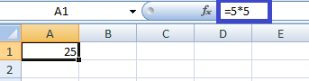
1. Asterisk Symbol

As previously explained, the asterisk symbol is used to multiply two numbers. The steps to be followed to perform multiplication in Excel using an asterisk are as follows:

1. Select a new cell, A1, and enter two numbers preceded by an equal sign.
2. Here the formula is written as =5*5.
3. Press Enter and the result will be displayed as 25.

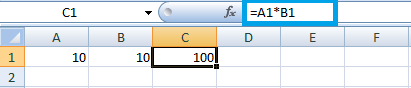
In this example, the numbers are entered by the user. What if numbers are already present in the cell for the given data?

To solve this problem, one can use cell names in the formula. The steps to be followed are as follows:

1. In the given data, the values are present in cells A1 and B1.
2. Select a new cell, namely C1, to display the result.
3. In cell C1, enter the formula as =A1*B1.
4. The result will be displayed in cell C1, the multiplication result of A1 and B1.

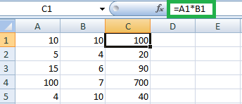
How to display the multiplication results for the columns of two data?

To display the multiplication results for the columns of two data, the steps to be followed are:

1. The given data contains the value of two columns, and the range is A1:B5.
2. To multiply the values in the two columns, select a cell, namely C1, to display the result and enter the formula as =A1*B1.
3. Press Enter. The multiplication value for cells A1 and B1 will be displayed in cell C1.
4. To get the result for the remaining data, drag the fill handle toward cell C5.
5. The multiplication result for the two columns will be displayed in column C1:C5.

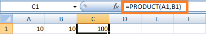
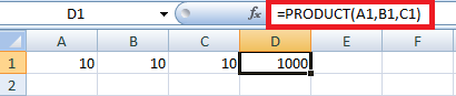
2. Product Function

As the name implies, the Product function is used to multiply two numbers. The steps to perform product function are as follows:

1. Enter the required data in the cell, namely A1 and B1.
2. Select a new cell, namely C1, to display the result.
3. In cell C1, enter the formula as =PRODUCT (A1, B1)
4. Press Enter. The Product function returns the multiplication value for the specified cell value.

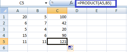
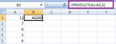
How to multiply two or more values using the Product function?

The data entered by the user contains two or more values. To calculate the multiple values using the product function, the steps to be followed are:

1. Enter the value in the respective cell, namely A1, B1, and C1.
2. Select a new cell where the user wants to display the result, namely D1, and enter the formula as =PRODUCT (A1, B1, C1).
3. Press Enter. The result will be displayed in cell D1, the multiplication result of three values.

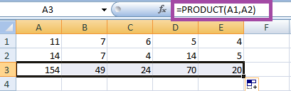
How to display the multiplication results for two data columns using the Product function?

To display the multiplication results for the columns of two data, the steps to be followed are:

1. The given data contains the value of two columns, and the range is A1:B5.
2. To multiply the values present in the two columns, select a cell, namely C1, to display the result and enter the formula as =PRODUCT (A1, B1)
3. Press Enter. The multiplication value for cells A1 and B1 will be displayed in cell C1.
4. To get the result for the remaining data, drag the fill handle toward cell C5.
5. The multiplication result for the two columns will be displayed in the column range C1:C5.

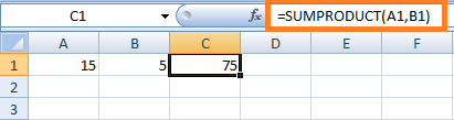
3. Sum product function

As the name implies, the sum product function multiplies the given values and adds the result. It multiplies the data present in ranges or arrays and sums the result. The range or array should be the same size or dimensions for the correct result. To multiply the values using the Sum product function, the steps to be followed are:

1. Enter the data in the worksheet, namely A1 and B1.
2. Select a new cell namely C1 where the result is displayed and enter the formula as =SUMPRODUCT (A1, B1)
3. Press Enter. The multiplication result of the required values will be displayed in the cell.

How to display the multiplication results for the columns of two data using the Sum-Product function?

To display the multiplication results for the columns of two data, the steps to be followed are:

1. The given data contains the value of two columns, and the range is A1:B5.
2. To multiply the values present in the two columns, select a cell, namely C1, to display the result and enter the formula as =SUMPRODUCT (A1:A5, B1:B5)
3. Press Enter. The sum of the product value for cells A1:A5 and B1:B5 will be displayed in cell C1.

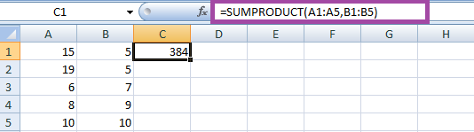
In the worksheet, the values present in range A1:A5 is multiplied by B1:B5, and the results are summed, which is displayed as 384.

Multiplication with Percentages

Multiplication with percentages converts the percentage into decimals and multiplying with the required number. The steps to multiply the number with percentage are as follows:

1. Enter the required number in cell A1 namely 11.
2. Select a new cell, namely B1, where the result is displayed, and enter the required formula in the cell as follows,

=11*5% in cell B1

=A1*0.05 in cell B2

=A1*5% in cell B3

3. Press Enter. The result for all three data will be similar, which is shown in the worksheet as follows,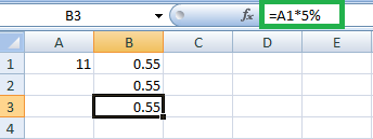

Multiplying rows in Excel

Based on the data requirement, the values are arranged in the worksheet. If the numbers present in the required rows wants to be multiplied using the respective formula, the values in the row are multiplied. Among the formulas explained, any formula can be used to multiply the numbers present in the row. The steps to be followed are:

1. Enter the values in the respective range of rows, namely A1:E2.
2. Select a new cell to display the result, A3, and use the required formula. Here the formula used is the PRODUCT function.
3. Enter the formula in C1 as =PRODUCT (A1,A2).
4. Press Enter. The result will be displayed in cell C1.
5. Drag the fill handle toward the cell to get the result for the remaining data.
6. E3. The result will be displayed in the cell range A3:E3.

How to multiply the rows of numbers with a specified number?

Method 1:

Multiplying the range of rows with a specified number is done using the respective formula. The steps to be followed are:

1. Enter the data in the required row, namely A1:A5
2. Select a new cell, B1, where the result is displayed, and enter the formula as =PRODUCT (A1:A5, 5).
3. Here A1:A5 is the cell range, and 5 is the specified number.
4. Press Enter. The result will be displayed in cell namely B1.

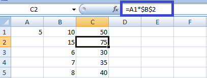
Method 2:

In Method 1, the multiplication number is entered directly into the formula. In Method 2, it is entered in the cell where the cell name is used as an absolute reference in the formula.

Absolute reference points to the same cell, whether copied or moved. The step to be followed to use absolute reference is as follows:

1. Enter the specified number in cell A1.
2. The respective values are entered in the column range B1:B5
3. Select a new cell to display the result, namely C1, and enter the formula as
4. = A1*$B$1.
5. Press Enter. The result will be displayed in cell C1. To get the result for the remaining data, drag the fill handle toward cell C5.

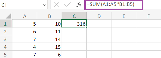
Multiplication in array

The value is entered in the array format in the formula for a larger data set. If the value is entered in array format, the large data set is calculated easily and quickly. In the multiplication concept, the data is entered in the format of the array, the steps to be followed are:

1. Enter the data in the cell range, namely A1:B5
2. To multiply and sum the data, enter the formula in the specified cell, namely C1, and enter the formula as =SUM (A1:A5*B1:B5)
3. Press Enter. The result will be displayed in the selected cell.

Similarly, the MAX, MIN, and AVERAGE values can be calculated using array multiplication.

The MAX value for the given data is calculated using the multiplication array as follows: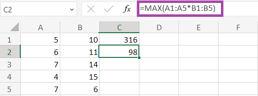

The MAX function calculates the value as 98 from the given data.

The Minimum function is calculated using the formula: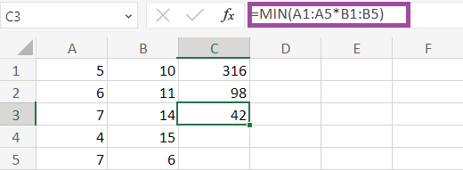

The MIN function calculates the values as 42 from the given data.

Summary

Multiplication plays an important role in calculating various data and real-time purposes. In Excel, multiple functions and methods are used to calculate the data quickly and efficiently, saving time. The different techniques are explained with examples in this tutorial. Based on the data, the required formula is used for the data.