| |

Excel PV FunctionMany of us buy insurance or invest in a company to secure a steady cash flow for our retirement years or any other future plans. Sometimes you also invest your money in FD with decent annual interest. Whatever the reason, there is always a second thought "is it a good deal?" To answer this question, the best way is to find the present value of your investment. Don't worry because Microsoft Excel has provided an inbuilt Excel function named PV function (it stands for "present value") to solve this problem. In this tutorial, we will cover the definition, syntax, and the steps to build correct PV formula for a series of cash flows, various examples, and more! What is PV Function?The Excel PV Function tells the present worth of the future payments (present value). PV function is categorized under Excel financial functions that return the present value of an annuity, loan, or investment based on a fixed rate of interest. The function was introduced with Excel 2007 and since then has been available in all versions, including Excel 2010, Excel 2013, Excel 2016, Excel 2017, and Excel 365. SyntaxParametersRate (required)- This argument represents the rate of interest per period. Nper (required) - This argument represents the total number of payment periods for the length of an annuity. pmt (optional)- This argument represents the payment made for each period. If this parameter is omitted, the default value is 0 but in that case the fv parameter must be included. fv [optional]: This argument represents the future value, or a cash balance the user want after the last payment is made. Since it is an optional parameter therefore its default value is 0. But if it is omitted in that case the pmt argument must be included. type [optional]: This argument provides the information regarding when payments are due.
Points to Remember about PV FunctionKindly have a look at the below given point to efficiently utilize the PV function in your worksheets and bypass common mistakes in Excel:
ExamplesExample 1: Calculate the present value of the annuity using PV function for the data given in the below table.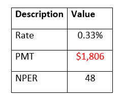
NOTE: In the above example, the pmt parameter is negative (represented by red) as we are investing the amount.To determine the present value of the annuity follow the below given steps: Step 1: Add helper row at the bottom of table Put your cursor below the table and add your helper row i.e., "Present Value". In this row we will type the PV formula and will fetch the periodic payment for the given data. Refer to the below image: 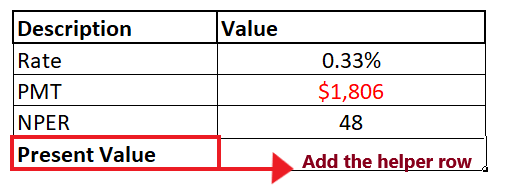
Step 2: Enter the PV formula Move to next cell of your helper row and start typing the formula = PV( It will look similar to the below image: 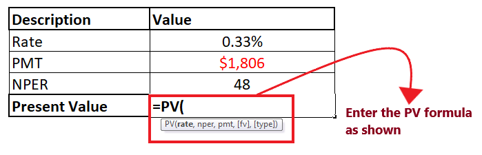
STEP 3: Add the parameter to your formula
The overall formula will look similar to the below image: 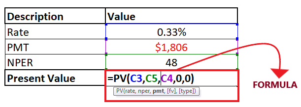
STEP 4: PV will return the output Press the enter button as soon as you are done typing the formula. Excel will return the output for your PV formula. As shown below it will return 79986 as an output of your periodic payment. Therefore, we can conclude that Present Value of 48 future payments of $1,806 is $79,986. 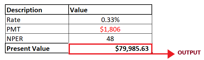
Example 2: Suppose you have invested in an insurance company where a regular payment of $200 is to be paid to the company at the beginning of every month for the next 10 years. The funding makes a 9% annual interest compounded monthly. Calculate how much the total annuity at the end of 10 years?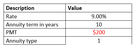
NOTE: In the above example, the pmt parameter is negative (represented by red) as we are investing the amount.To determine the total annuity at the end of 10 years the below given steps: Step 1: Add helper row at the bottom of table Put your cursor below the table and type the heading of your helper row i.e., "Present Value". In this row we will type the PV formula and will fetch the annuity worth for the given data. Refer to the below image: 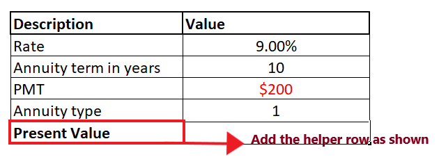
Step 2: Enter the PV formula Move to next cell of your helper row and start typing the formula = PV( It will look similar to the below image: 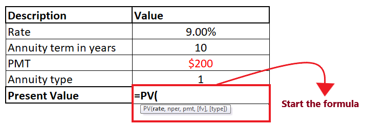
STEP 3: Add the parameter to your formula
NOTE: Always remember to convert annual interest rate to periodic interest rate while working with Excel PV formula for monthly cash flows.
The overall formula will look similar to the below image: 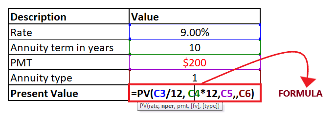
STEP 4: PV will return the output Press the enter button as soon as you are done typing the formula. Excel will return the output for your PV formula. As shown below it will return 15,906 as an output of your periodic payment. Therefore, we can conclude that the annuity worth will be 15,906.7 at the end of 10 years. In the above example, we calculated the yearly annuity. Similarly, you can find the present value for a weekly, quarterly, or semiannual annuity. To achieve this, you only need to change the number of periods per year in the respective cells: 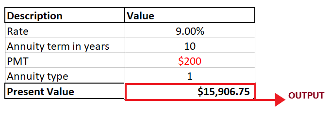
Next TopicHow to go to next line in excel
|
 For Videos Join Our Youtube Channel: Join Now
Feedback
- Send your Feedback to [email protected]
Help Others, Please Share


