| |

Excel Transpose FunctionWhile working with Excel, many times, you require switching or rotating cells in your worksheet. The hard way of achieving this is by copying, pasting the data to the required cells. This way, it is time-consuming. The other way round of switching and rotating your cells is using the Excel Transpose function. But this function formulates duplicated data. If you don't want the duplication in your worksheet, you can type a customized formula instead of using the inbuilt TRANSPOSE function. For instance, in the following reference image, the function =TRANSPOSE (A24:B44) takes the range of cells A24: B27 and organizes them horizontally (refer to the below screenshot). 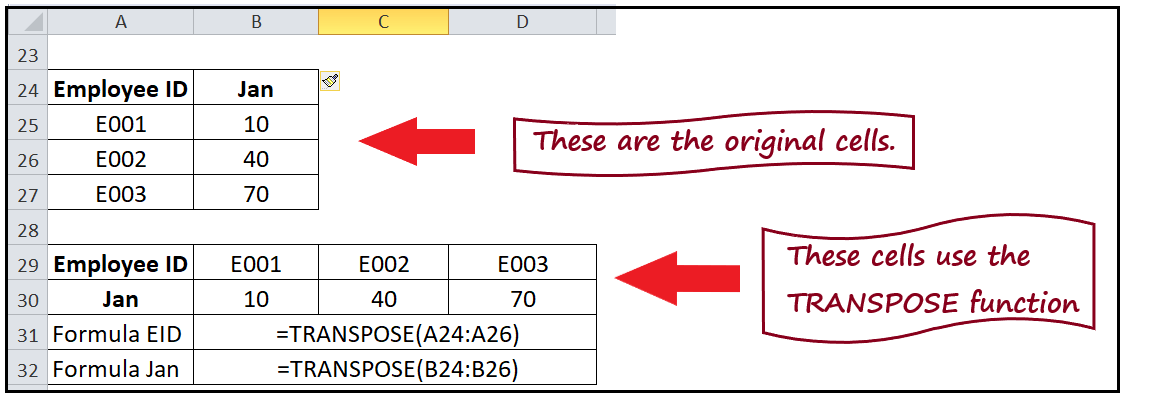
What is TRANSPOSE function?The Excel TRANSPOSE() function copies the data vertical range of cells to a horizontal range of cells, or vice versa (i.e., changes the orientation of horizontal range to vertical range range). In simple terms, we can say this function "flips" the placement of a given range of cells or Excel array:
In other words, when an array is transposed, the first row is flipped, and it becomes the first column of the new array; similarly, the second row of the previous array becomes the second column of the new array, the third row will be converted as the third column, and so on. In Excel, the TRANSPOSE() function can be used with both cell ranges and arrays. Though users prefer the use of Transposed ranges as they are dynamic, i.e., if data in the original range changes, the TRANSPOSE() data will immediately update data in the new range. Syntax
=TRANSPOSE (array)
Parametersarray (required) - This parameter represents the data which you want to change from vertical to horizontal or vice-versa. Return ValueThe TRANSPOSE function returns a range of cells or array by converting the horizontal range of cells as a vertical range or vice versa. Steps to use the Transpose Function
Example 1: Use TRANSPOSE function to change the cells from vertical to horizontal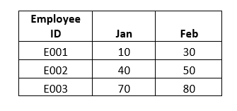
Follow the below steps to solve the above problem: Step 1: Select blank cells same size as the original rangeThe first step is to select blank cells the same size as the original range in your Excel worksheet. But always remember to select the same size cells in the other direction. For instance, in the below example we have twelve cells here that are arranged vertically: 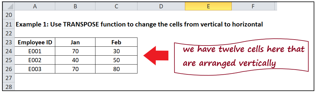
So, we will select twelve horizontal cells, as shown in the below image: 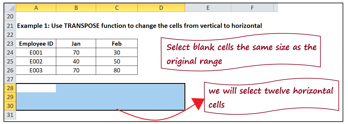
These blank cells are the location where are transposed cells will be placed afterwards. Step 2: Type the formula i.e., =TRANSPOSE(After you select the blank cells, just type the formula: =TRANSPOSE( It will look similar to the below image: 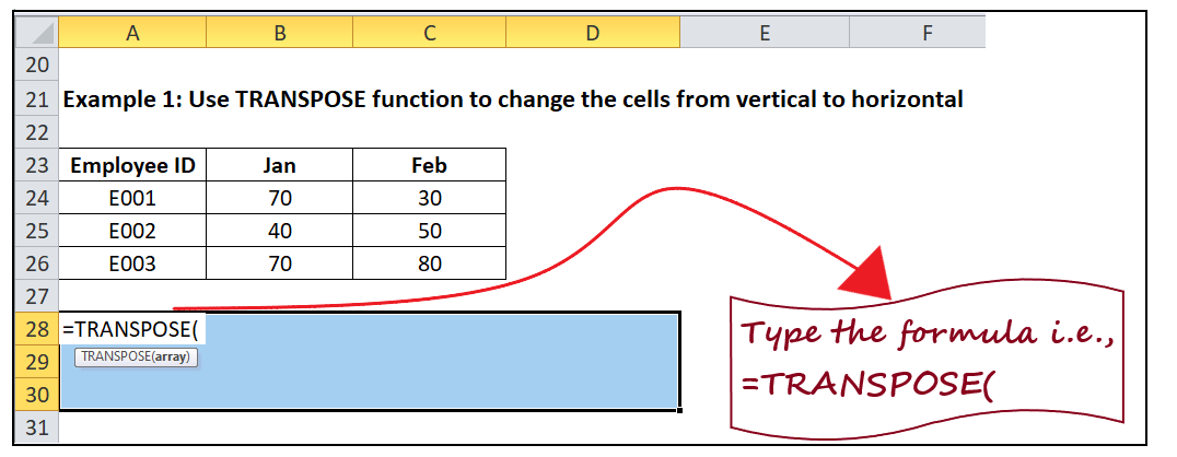
NOTE: You will notice that those nine horizontal cells are still selected in your Excel worksheet even though you have started typing the TRANSPOSE function. Step 3: Enter the range of cells you wish to transposeThe next step is to type the range of the cells you want to transpose. Although instead of typing you can point and drag your mouse cursor to select the group of original cells. In this example, the original cells are positioned from A23 to C26. Therefore our formula becomes: =TRANSPOSE (A23: C26). After entering the range you will notice that the entire array is highlighted with a blue rectangle box. It will look similar to the below image: 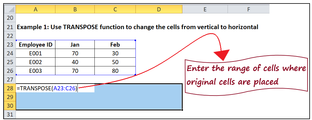
NOTE: After typing the formula keep in need that you don't press ENTER yet as it will show the #VALUE error. Stop typing, and move to the last step. Step 4: Press CTRL+SHIFT+ENTER togetherThe last step is to press CTRL+SHIFT+ENTER keyboards buttons together and Excel will immediately transpose the original cells for you. Below given is the output after transposing the original cells using TRANSPOSE() function. 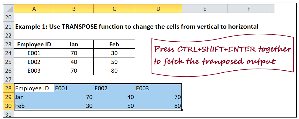
NOTE: You will notice that curly brackets are automatically added to the beginning and end of your TRANSPOSE formula, to indicate that it is array function.Question: Now the question arises why it only works by pressing CTRL + SHIFT +ENTER?Answer: The answer to this question is because the TRANSPOSE function is only used in an array formula, and that's how you terminate an array function. An array formula is applied to multiple cells. If you recall, in step 1, you have selected multiple cells; therefore, the formula will be applied to more than one cell. Example 2: Change Orientation of a 4 row x 6 column Dynamic Array (given below) using the TRANSPOSE function.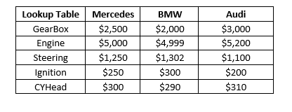
Follow the below steps to transpose the above 4 row x 6 column Dynamic Array : Step 1: Select the blank cellsTo transpose a 4 row x 6 column horizontal range to a 6 row x 4 column vertical range select 24 blank cells (6 row and 4 columns). In this example, we have selected the range of cells B4:C7. 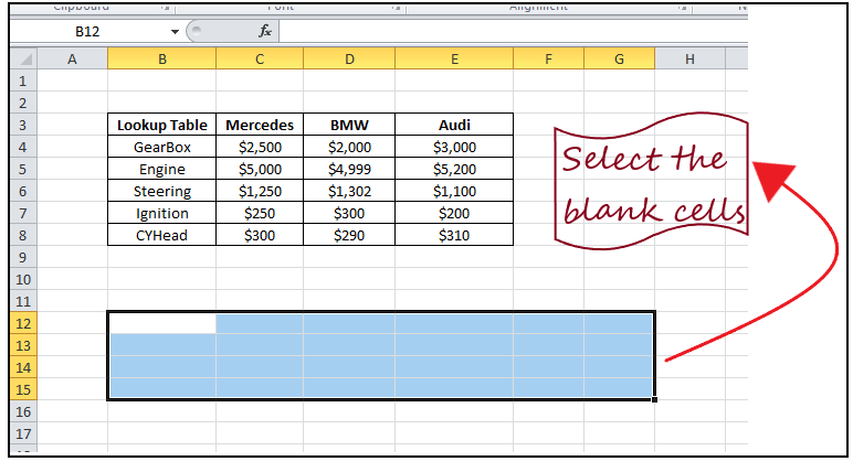
Step 2: Type the formula and enter array of range of cellsAfter selecting the blank cells, just type the formula and select the range of cells you flip. You will have the following formula. =TRANSPOSE(B3:E8) NOTE: As soon as you type the formula you will notice a night blue rectangle box covering your array.It will look similar to the below image: 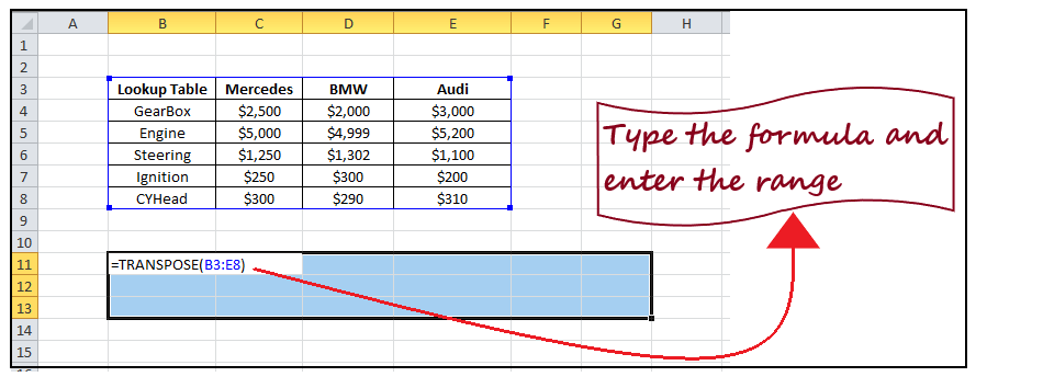
STEP 3: Press Ctrl+Shift+Enter to fetch the outputThe last step is to press CTRL+SHIFT+ENTER keyboards buttons together and Excel will immediately transpose the 4 row x 6 columns original dynamic array to 6 row x 4 column range of cells. It will look similar to the below image: 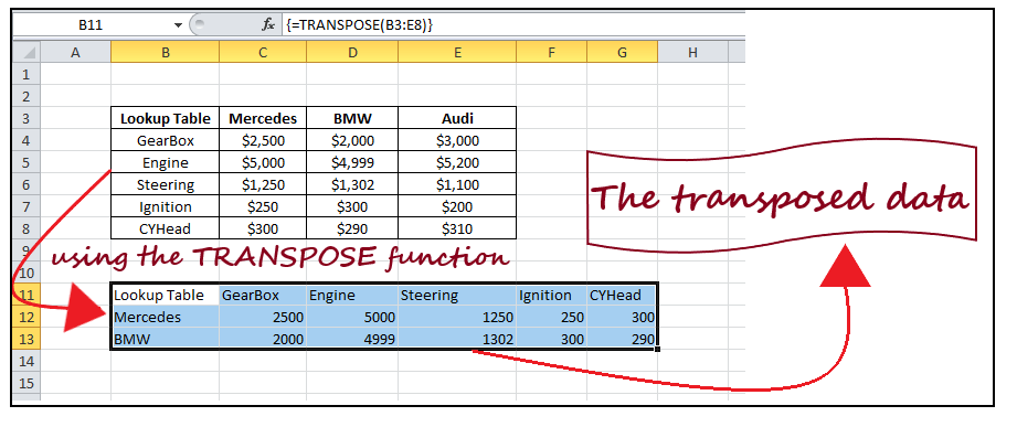
Eureka! Now we have understood how the TRANSPOSE function works in an Excel worksheet. You can also integrate this function with other Excel formulas. Go ahead and give it a try. Points to Remember
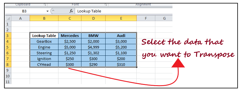
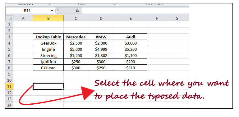
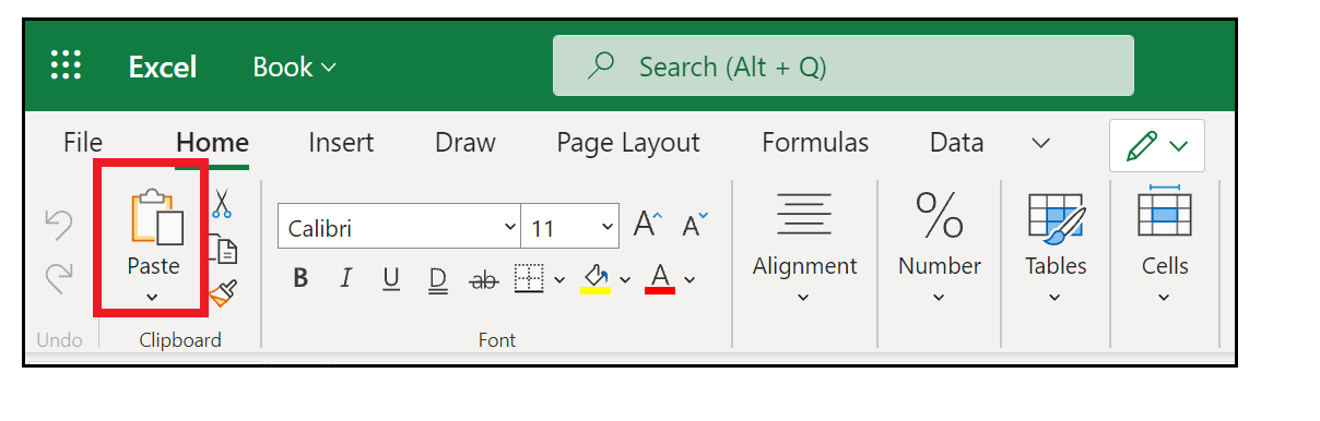
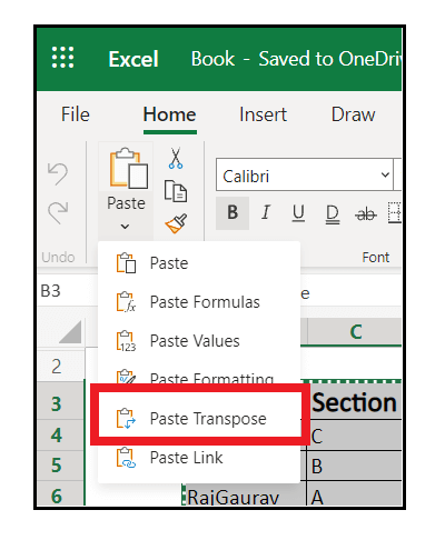
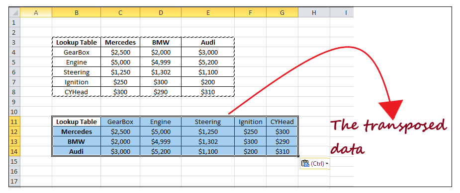
TRANSPOSE Alternative- Paste Special OptionThe TRANSPOSE function is logical when you require a dynamic solution that will automatically update the flipped output whenever there is any change in the original data. However, Excel provides an easy alternative to the TRANSPOSE function, i.e., the Paste Special Option. It can be very useful when you only need a one-time conversion. You can use Paste Special and can easily flip the worksheet data's orientation without keeping a link to the source data. Follow the below steps to use the Paste Special option to transpose your worksheet data:
NOTE: Make sure to select a single cell or a group of cells to paste the transpose data. IF the cursor is over the source data cells, Excel will throw an error that, "The information cannot be pasted because the copy and paste area are not same size and shape"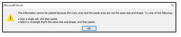
Next TopicCircular reference in Excel
|
 For Videos Join Our Youtube Channel: Join Now
Feedback
- Send your Feedback to [email protected]
Help Others, Please Share


