Custom Number Format in Excel

MS Excel or Microsoft Excel is powerful spreadsheet software developed by Microsoft by combining all the necessary features, functions, and tools. When it comes to formatting data within a spreadsheet, Excel has several formatting options to format different types of values accordingly. One of the essential features in Excel is to use number format, which enables us to format any numerical value entered within cells. Excel has a wide range of built-in number formats. As a bonus, it also supports custom number formats.

This article discusses the Custom Number Format in Excel and the required steps to apply it to our Excel sheets. Before discussing the custom number format in Excel, let us first understand the quick introduction of Excel Number Format:

What is Number Format?

A number format in Excel refers to a specific code or format that controls the way values are displayed within Excel cells. Excel has several inbuilt formats to help us display values in different ways in spreadsheets for Number, Percentage, Currency, Accounting, Date and Time, etc.

Example: The following table displays different formats of the same date based on the given or applied code:

The main purpose of the number format is to change the way numerical values are displayed. This does not affect the actual value in the cell, and we can still do the relevant calculations accordingly. In short, the underlying value recorded within the cell is not changed.

What is Custom Number Format?

Although Excel consists of several inbuilt formats, there may be cases when we want to use our specific format, called custom format. Excel is a powerful tool, and we can create our custom number format. It helps us control the execution of numerical values within the spreadsheet as per our choice. Excel enables users to leverage multiple formatting options that get auto-applied on the desired or selected cells with custom formatting.

For example, we might need to automatically format the number 283020000 as $283.02M using the custom number format. Similarly, we may need to format a single-digit value to five digits, even if we only enter a number. Instead of typing 00001, we can set a custom format and enter 1, and leading zeros will be added automatically by Excel.

Where can we use custom number formats?

We can use custom number formats in many areas within the Excel workbook. It is easy to use them in charts, tables, formulas, pivot tables, and worksheets.

• When using custom number formats in worksheets, we apply them from the Format Cells dialogue box.
• When using custom number formats in Pivot Tables, we apply them from value field settings.
• When using custom number formats in Charts, we apply them using data labels and axis options.
• When using custom number formats in formulas, we apply them with the help of the TEXT function.

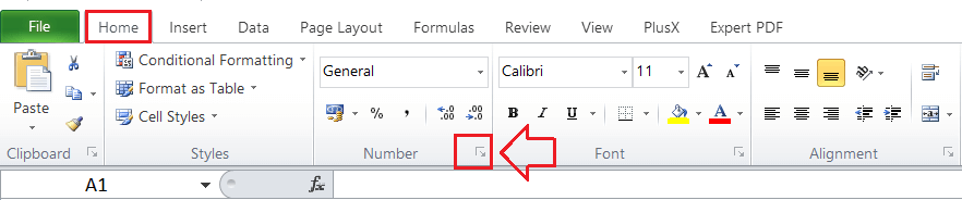
How to access Number Formats in Excel?

To access the number formats in Excel, we need to navigate the Home tab and locate the 'Number' group. It looks like this: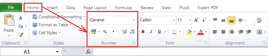

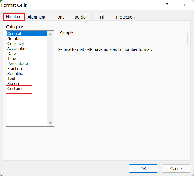
In the above image, these are the built-in number formats. We can click the drop-down icon next to 'General' to access all the common number formats. However, we need to go to the Format Cells dialogue box to access more number formats.

Note: By default, Excel applies different number formats automatically on values that we enter within the cells. For instance, if we enter a valid date in an Excel cell, its format will automatically change to the default 'Date' format. Similarly, when we type a value in percentage like 10%, it will be changed to percentage, and so on.

How to create a custom number format in Excel?

To access all the number formats in Excel or to create custom number formats, we need to follow the below steps:

• First, we need to select or highlight all the cells we are willing to apply the number format or custom number format.
• Next, we need to launch the Format Cells dialogue box. For this, we need to click on the More button from the Home > Number group, as shown below:
  
  Alternately, we can use the keyboard shortcut 'Ctrl + 1' to open the Format Cells dialogue box quickly.
• In the Format Cells dialogue box, we need to select the Number tab if not selected. Under the category option, we can access all the available number formats of Excel. We must click the Custom option to create our desired number format.
  
• In the next window, we need to enter the format code under the Type box, and it will be applied to selected cells. The format code must be typed with proper structure.
  
• After entering the desired format code, we must click the OK button to save the newly created format.

Structure and Reference of Excel Number Format

To create a custom number format in Excel, we must know the proper structure of the number format that Microsoft Excel follows. An Excel number format mainly contains the following four sections, divided by semicolons in a sequence:

The following code is the typical example of a custom format in Excel: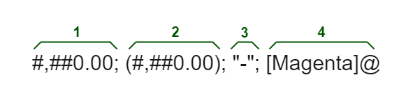

Where,

1. It denotes the formatting for the positive numbers. Our example will display values at 2 decimal places and a thousand separator.
2. It denotes the formatting for the negative numbers. It is almost identical to positive numbers; however, it is enclosed within the parenthesis.
3. It denotes the formatting for zeros. In the above example, it will show dashes instead of zeros.
4. It denotes the formatting for text values. In above example, it will show text in magenta font color.

However, the Excel Number Format can have up to four sections. But, only one section is mandatory.

Important Rules for Custom Number Format

To create a custom number format without errors, we must remember the following rules:

• If we enter only one section in custom number format, the format is applied to all the number types, such as positive, negative, and zeros.
• If we enter two sections in custom number format, the first section is applied to positive numbers and zeros, while the second section is applied to negative numbers.
• A custom number format must contain all four sections to apply the given format to text values.
• If we want to use the default number format for any middle section, we can type General instead of entering the corresponding format in our custom number format. For example: General; -General; "-"; General. Here, we have added the minus sign in the second section as the second section denotes the formatting for the negative numbers.
• Excel also allows us to edit the built-in Excel format. However, the copy of the edited format is created while the original number format remains intact from the customizations.
• To hide any desired section or value type(s), we can skip the specific section in custom format by typing only the ending semicolon. For example- General; ; ; General. The negative value and zeros will only be displayed in the formula bar, not within the cell area.

Digit and Text Placeholders for Custom Number Format

Some characters in custom number format codes have specific meanings. They generally act as building blocks and can help us create an infinite number of formats. The following table displays the most common formatting codes and their uses:

Theoretically, there are infinite numbers of Excel custom number formats that we can create using a predefined set of formatting codes listed in the table above.

Excel Custom Formatting Guidelines

The following tips or guidelines explain the most common and useful implementations of predefined format codes in Excel:

Decimal Places in Custom Number Format

We can control the number of decimal places using the custom number format. The decimal point location is displayed in Excel number format by a period (.). Besides, the desired number of decimal places is controlled using zeros (0). For instance:

• We can use 0 or # to show the nearest integer without decimal places.
• We can use 0.0 or #.0 to show the nearest integer with one decimal place.
• We can use 0.00 or #.00 to show the nearest integer with two decimal places, and so on.

The primary difference between 0 and # in the integer part of the format code is that when we use the pound sign (#) to the left-hand side of the decimal point, numbers less than 1 start with a decimal point. For instance, when we use the format code #.00, the given number 0.25 is displayed as .25. However, the 0.00 format displays the given number as 0.25.

The following sheet displays a few more examples of custom number formats in relation to the general format: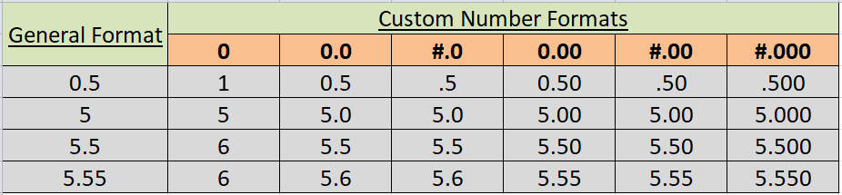

In the above example sheet, it is important to note that the digit placeholders work by following these principles:

• Suppose the number within the cell has more digits to the right side of the decimal point than the placeholder in the applied format. In that case, the number is automatically 'rounded' to as many decimal places as the placeholder. That's why the number 5.55 with format 0.0 has become 5.6 in the above example sheet.
• All the digits placed left side of the decimal point display the value regardless of the number of placeholders. The number 505.55 with the format #.# will be displayed as 505.6.

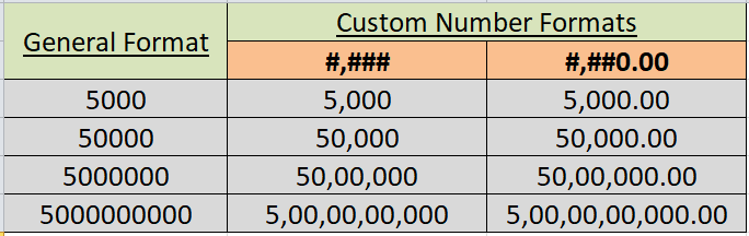
Thousands Separator in Custom Number Format

We need to use comma (,) within our custom number format or code to include a thousand separators. For instance:

• We can use #,### to show a thousand separators without decimal places.
• We can use #,##0.00 to show a thousand separator with two decimal places, and so on.

Large Numbers in Custom Number Format

As discussed above, we can use one comma (,) to display a thousand separators. Likewise, we can use two commas (,,) to display millions. For instance, we can use the format 0.0,, "M" to display one decimal place and the letter M next to the given value to denote million.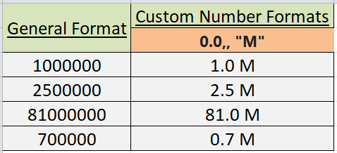

Leading Zeros in Custom Number Format

By default, when we enter numbers like 05 or 0005 in cells with General formats, Excel automatically removes the leading zero and changes the value to 5. Technically, all three values are the same. However, sometimes, we may need numbers with the desired numbers of leading zeros.

The typical method to enter the desired value with leading zeros is to use the apostrophe (') before the value. This means that we need to enter '05 or '005, and the value will be treated as a text string, preserving leading zeros in a cell.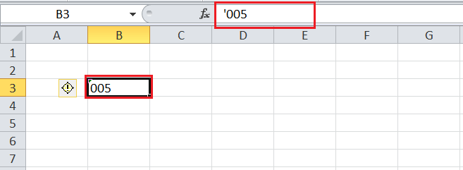

When we want to include specific numbers of leading zeros with many values in a column, it is easy to use a custom number format. As discussed above, zero (0) is the placeholder used to display insignificant zeros. Therefore, if we want to enter numbers up to 7 digits with leading zeros when needed, we can use the custom format code as 0000000 in corresponding cells. After that, if we enter just 5, the value will be displayed as 0000005.

The following sheet displays a few more examples:

Percentages in Custom Number Format

If we want to display the number as a percentage of 100, we must use the percentage sign (%) within the format. For instance:

• We can use the format #% to show percentages as integers.
• We can use the format #.00% to show percentages with two decimal places.
• We can use the format #,##.00% to show percentages with two decimal places and a thousand separators, and so on.

The following sheet displays a few examples of the above-listed number formats in relation to the general format: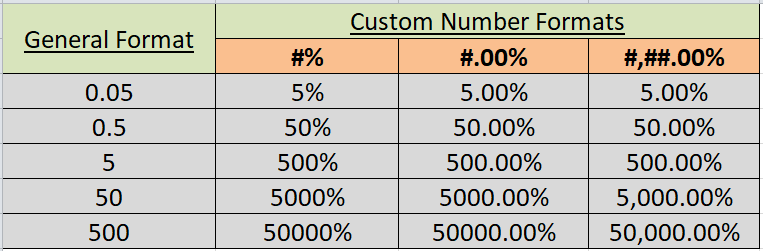

Repeat Characters in Custom Number Format

If we want to repeat any specific character to fill the cell width, we need to include an asterisk (*) before the character. For instance:

• We can use the format #*= to automatically insert equal signs after the given value to fill the cell width.
• We can use the format *0# to add leading zeros before the given value.
• We can use the format @*- to add dashes after the given text value. The @ symbol is used to input text values.

The following sheet displays a few examples of the above-listed number formats in relation to the general format: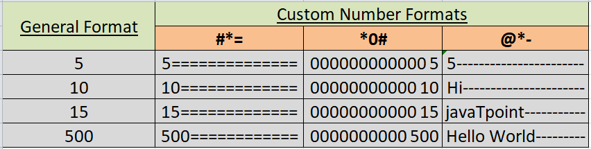

Colors in Custom Number Format

Excel also enables users to change font colors for specific value types within the cells. Technically, Excel supports only 8 built-in colors. If we want to use any of the built-in colors in our fonts, we need to type a particular color name in the desired section of the custom format code. But, the color name must be entered as the first item of the specific section.

The supported colors are listed in the following table:

For example, if we want only to change the font color but leave all the default or General formats intact, we must use a format similar to this:

We can also control the formats in each section and combine the color format with them all simultaneously. For instance:

The above format will display general values with colors and applied formats, e.g., display the 2 decimal places, a thousand separator, and show zeros as dashes: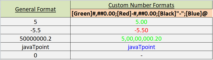

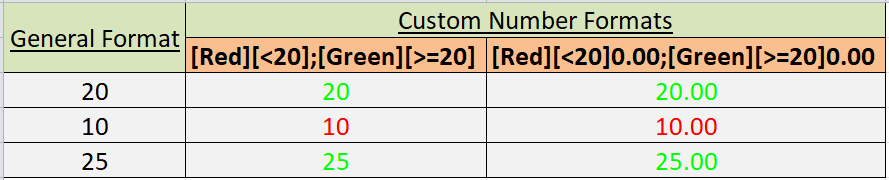
Conditions in Custom Number Format

We can also apply the desired formats based on specific conditions. This means we can input conditions, including the comparison operator and a value, and enclose them in square brackets []. The square brackets here represent the conditions. For instance:

• We can use the format [Red][<20];[Green][>=20] to show red color when the given numbers are less than 20 and the green color when the numbers are greater than or equal to 20.
• Likewise, we can use the format [Red][<20]0.00;[Green][>=20]0.00 to show two decimal places with the above condition, as shown in the following image:

Dates and Times in Custom Number Format

Excel date and time formats are based on a specific case with unique format codes. They are not easy to manipulate as many dates and time formats exist. However, we can control dates and times using the custom number formats.

For example, suppose we apply the long date format in cell A1 and enter the date as 01-01-2021. It will be displayed as: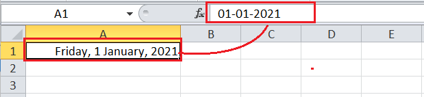

Now, we need to click the OK button and apply the custom number format in the same cell as mm/dd/yyyy, dddd.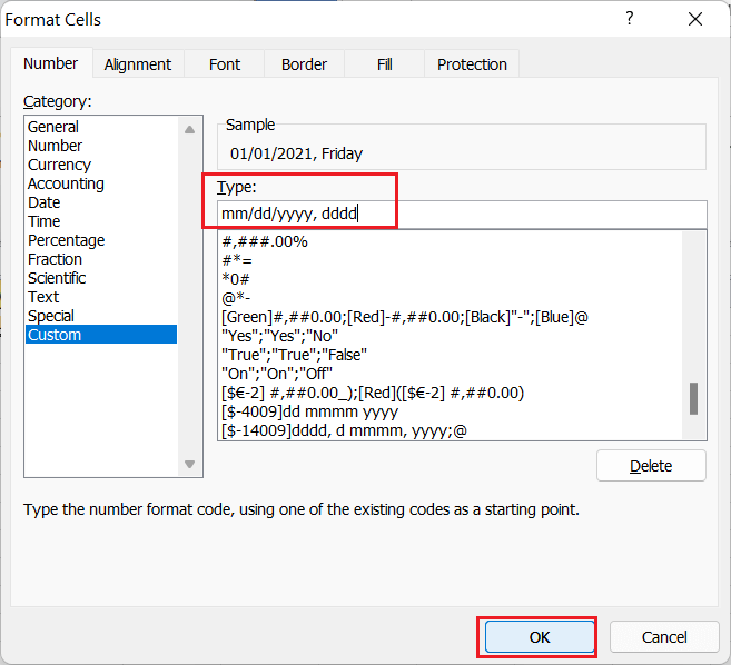

Now, the date will be displayed as below: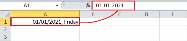

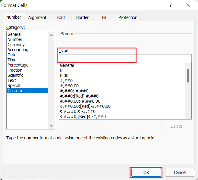
Deleting a Custom Number Format

If we don't want to use any created number format (custom number format) in the future, we can delete that specific format from the list. For this, we need to go to the Format Cells dialogue box, choose Custom under the Category, locate or enter a specific format/ code in the Type list, and click on the Delete button.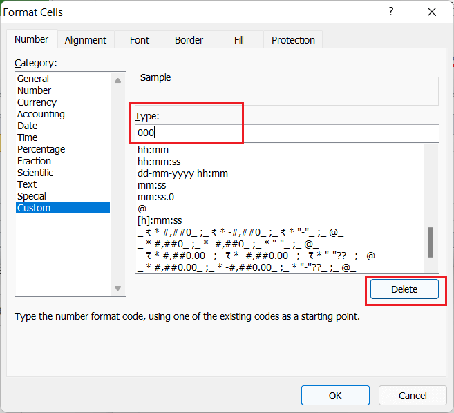

Despite this, the custom number format is stored within the workbook where we apply it. Therefore, if we want to use the same custom formats in another workbook, we must copy the corresponding cells from one workbook to another. That way, the same custom number formats will also be available in a particular workbook.