How to change the row color in Excel based on a cell's value

Microsoft Excel allows changing the row colour based on the cell's value, and it is often required to highlight the cell based on its value.

In this tutorial, we will cover the different methods, tips and formula examples to highlight entire rows filled with number and text values. We will be covering the below topics:

1. Changing the colour of a row based on a number for a single cell
2. How to add multiple rules with the priority you need
3. How to change a row colour based on a text value in a cell
4. Change a cell's colour on the basis of another cell value

Let's get started!

Steps to change the colour of a row based on the values of a single cell

We are given the following data, and are asked to shade the cells.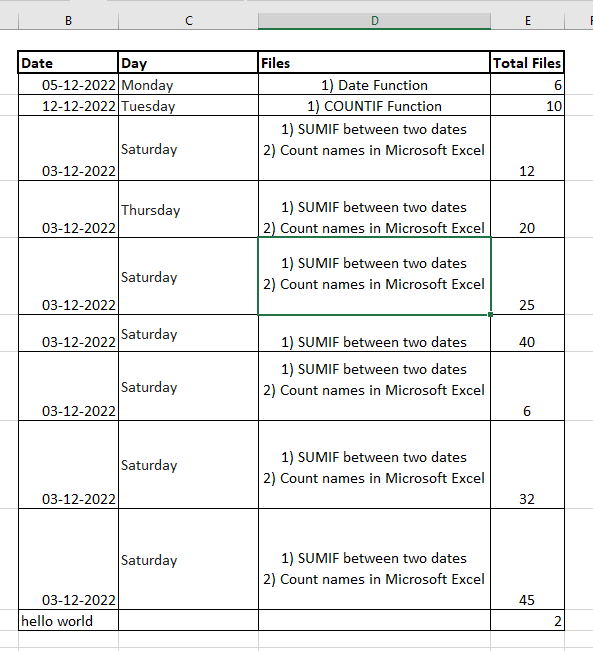

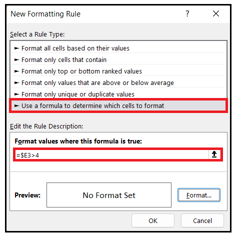
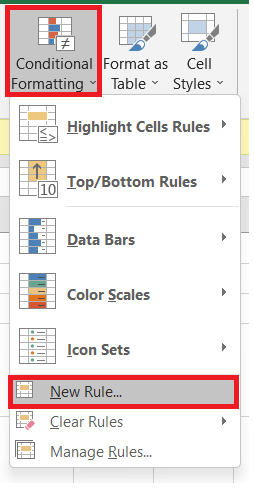
To distinguish between the values many times, we shade the rows (Carrying distinct values) with different colours. It helps end users instantly determine the values and see the most important orders at a glance. Now the question arises of how to get it done in Excel, and the solution to this problem is Conditional Formatting.

Perform the following steps to quickly change the row colour based on a number for a single cell:

1. The first step is to select the cells for which you want to change the background colour.
   
2. We will create a new formatting rule. To enable this, go to the Home tab, click on the Conditional Formatting > New Rule...
   
3. The "New Formatting Rule" window will appear. Select the option "Use a formula to determine which cells to format" and add the formula .This will help to highlight the cells where the total files number are greater than 15. Refer to the below formula.
   =$F3>15
   
4. You can alter and put your own formula using the less than (<) and equal to (=) operators. You can highlight values smaller than 10 or even equal to 10.
   =$F3<10
   =$F3=10

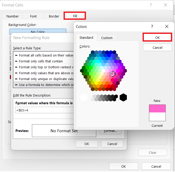
Note: Make sure to put the dollar symbol $ before the cell's address, and it will ensure that the same column letter persists when the formula gets copied across the row. It's the only trick you must remember to apply the formatting to the whole row based on a value in the selected cell.

1. The last step is to apply a format to the filtered cells. From the bottom of the window, click on the "Format..." option and move to the Fill tab to change the background colour of the cells. Select from the given colour range and if none match your liking, click on the "More Colors..." option to select the one you like, and click on the OK button.
   
2. The rows where the number of files were greater than 15 will get coloured. You will have the following output.

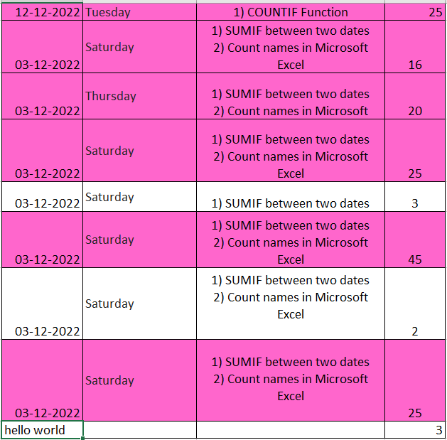
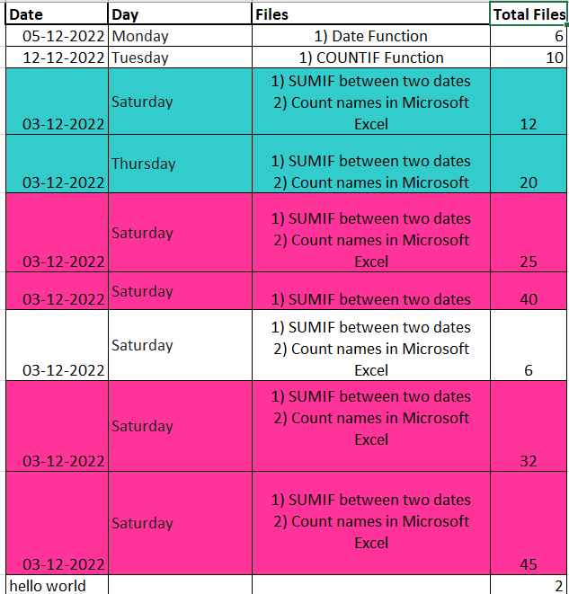
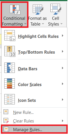
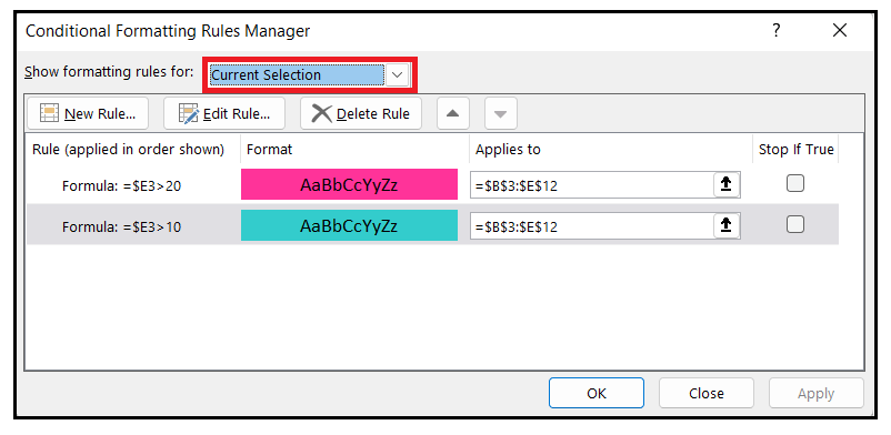
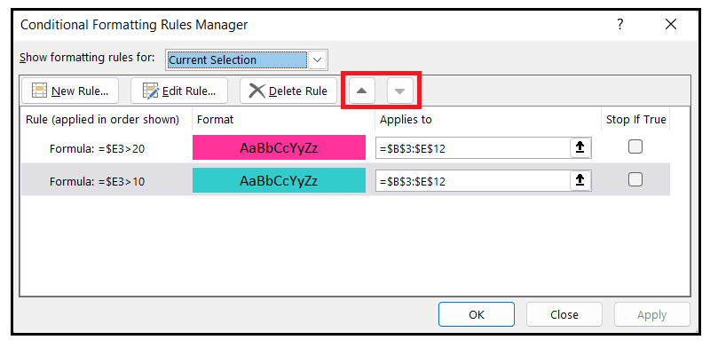
Filling out cells with a single colour is easy. Now let's move forward and add multiple rules within a selected range of cells.

How to add multiple rules with the priority you require

In the previous example, we highlighted the Excel rows with single colour based on values in the Number of files field. Now, if you want to apply a second rule in the same dataset where we want to change the colour of the cells if the value is greater than 20, for instance, you can apply a rule to colour the rows that contain the quantity 10 or greater. Use the below formula to get it done!

=$F3>10

Once you have created the second formatting rule, we need to set the priority using the following steps:

1. Go to the Home tab, from the Styles group, click on the Conditional Formatting option. The following dialog window will pop-up, click on the Manage Rules....
   
2. Choose "This worksheet" in the "Show formatting rules for" field. Since in our case, we want to manage the formatting rules only the current selected cells, therefore we have chosen "Current Selection" option.
   
3. Position the formatting rule as per the priority you require. For instance, position the one you want to apply first to the top using the arrows. The output is shown below:
   
4. Once done, click on the OK button, and the selected rows will immediately modify their background colour based on the set priority that you have specified in the above formulas. Refer to the below image.

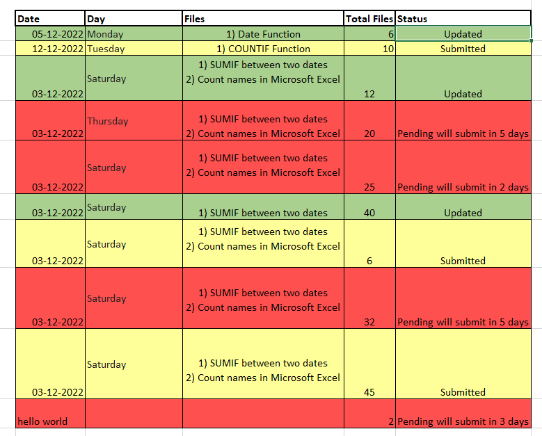
How to change a row color based on a text value in a cell

So far, we have applied conditional formatting to the cells based on numbers. You can easily apply conditional formatting based on text values as well. For instance, in the following table, you can highlight the cells based on their delivery status so that:

• Change the background colour of the cell to green if it contains text value "All the files are updated"
• Change the background colour of the cell to yellow if it contains text value "All the files are submitted"
• Change the background colour of the cell to yellow if it contains text value "Some files are pending"

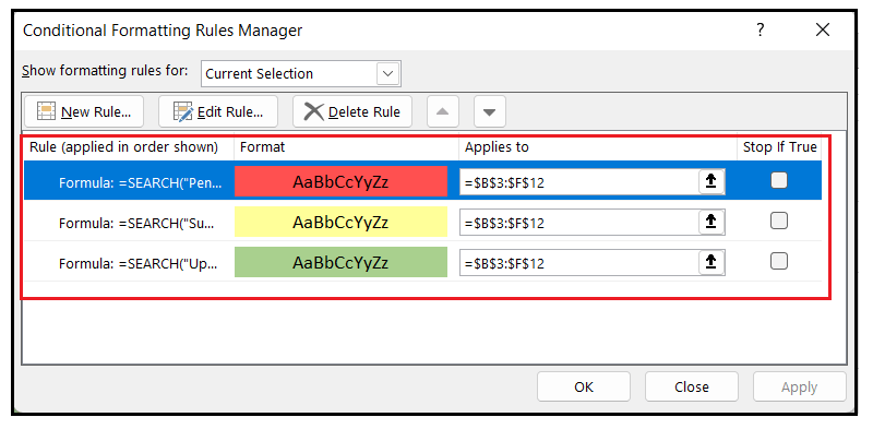
Now the question arises of how to implement the above logic in a formula. If we apply a formula using the direct keywords like "Updated" (=$F3= "Updated"), "Submitted" (=$F3= "Submitted") or "Pending" (=$F3= "Pending"), the formula won't give the desired results. It's because the above formula starts looking for an exact match, and our text contains more text; therefore, an exact match won't give what we want.

In such cases, the best method is to take advantage of the Search function that works for the partial match as well. Perform the following steps to quickly change the row colour based on the partial match:

1. Go to the Home tab, from the Styles group, click on the Conditional Formatting. The dialog window will appear, click on the New Rule....
   
2. The "New Formatting Rule" window will appear. Select the option "Use a formula to determine which cells to format" and add the formula in the "Format values where this formula is true" field. Using the format option change the colour of the cells to green.
   =SEARCH("pending will", $F3)>0
3. Apply the two more formula for pending and submitted files and change their background colours to red and yellow respectively. Click on Ok button to apply the formatting rules to the selected cells.
   
4. The cells will change their colour as per the status of the files. You will have the following output.

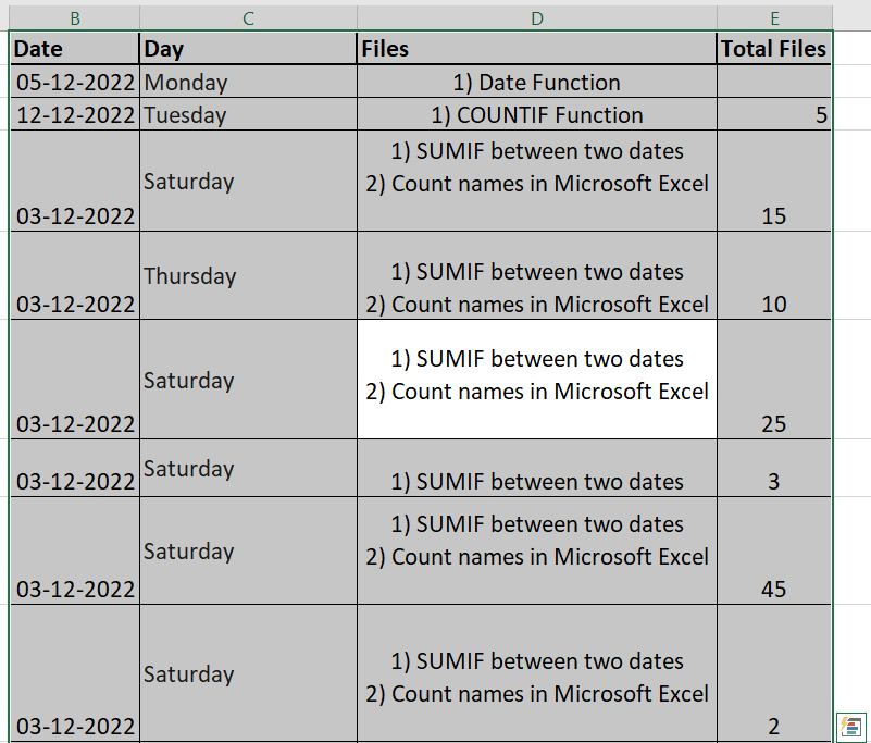
Easy Isn't it!

Highlight row if cell starts with specific text

If in the formula we use >0, it represents that no matter what text value we supply, the specified row will be coloured. For instance, the column (F) contains the value "status", since the key value is greater than 0, therefore this row will be coloured.

Now, we can modify the formula where the row will be coloured only if the key cell starts with a given text, and to implement this we will use =1 in the formula,

The above formula represents that the row will only be highlighted if the given text is found at the first position of the specified text in the cell.

NOTE: Sometimes, if you text contains leading spacing, in such cases this formula may not work properly. Therefore, ensure that there are no leading spaces present in the key column, else the formula will not return an optimal solution,

How to change a cell's color based on another cell's value

It's a simple and easy variation of changing a cell's colour based on another cell's values. It is mostly useful when instead of changing the entire dataset, you choose to select the background colour of some specific column or range of cells.

For example, we could create the above formula rules only, but instead of shading the entire dataset, we can specify only column D (Files field), where column D will be shaded based on the status of the files.

Rest all the steps will remain the same; all you need to do is to apply it only to cell D3 to D12.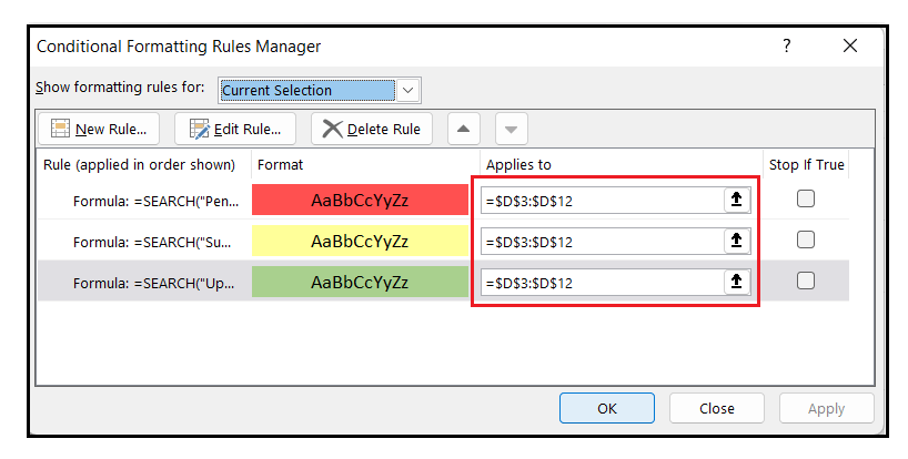

The above sequence of formula will return the following output where only the cells column D is shaded based on the values of column F.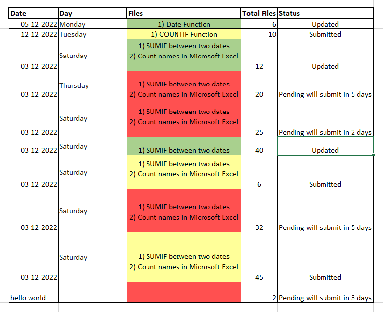

Conditional Formatting is an amazing Excel tool that quickly helps to highlight cells on the basis of any criteria that you want to apply. We have already covered some interesting formulas in this tutorial. Go and give it a try today!