What is meant by Conditional formatting in Microsoft Excel

It was well known that the respective "Conditional formatting" in Microsoft Excel is primarily a tool that applies formatting to our data, which depends upon the various conditional rules we usually lay out.

Moreover, Conditional formatting is a unique formatting feature of Microsoft Excel that is effectively used to find unique and duplicate values by just formatting the cells. And this particular feature is available in various spreadsheet applications in which, Microsoft Excel is one of them.

And Conditional Formatting in Excel sheets can be efficiently used in several ways, that will include the following ones:

• It helps in the visualization of the data our data.
• It also helps in checking for specific information.
• And it is, additionally, a great way to highlight top values or differences in our data as well.

Besides all this, "Conditional Formatting" enables the different features to the users to make the data more informatic and readable as well. It also allows us to format the cells and their data effectively, which will meet the specified criteria respectively.

Now in this chapter, we will be learning about the several uses of conditional formatting and how it applies to an Excel worksheet to make out the data more useful.

Topics covered in this chapter

The following list of topics, which we are going to cover in this chapter as well-

• Features of conditional formatting
• Where the conditional formatting option is available?
• Conditional formatting Basics
• Pre-set conditional formatting
  • Highlight Cell Rules
  • Top/Bottom Rules
  • Data Bars
  • Color Scales
  • Icon Sets
• Highlight the cells
• Apply data bars on data
• Apply color scales on data
• Clear conditional formatting
• Define Custom Conditions (new rules)

Features of the conditional formatting

It is well known that the respective Microsoft Excel enables different features of conditional formatting, which are as follows:

1. We can easily highlight the various cells with a background color to make the data more valuable and efficient.
2. With the help of this, we can also format the various cell content with a particular type of font as per our requirements.
3. It allows us to format the cells and their data that will effectively meet the desired criteria.
4. Microsoft Excel allows an individual to put conditions on data and format the cells based upon the following conditions, greater than, less than, duplicate values, unique values, and equal if Text containing specified data.
5. We can also set out the rules to format the data and transparent the rules we set either from selected cells or the entire sheet earlier.
6. Conditional formatting enables us to perform several things with data, like we can set the icons with the data, such as indicators, shapes, directional, etc.
7. Conditional formatting makes the data more readable and informatics to the reader for the analysis purpose.
8. For the analysis purpose of the spreadsheet, conditional formatting is an excellent choice to format the data.

• Note: When to make Use of the conditional formatting in Microsoft Excel?
  We can efficiently use the conditional formatting in Microsoft Excel to visualize month-over-month marketing statistics, highlight the link-building opportunities by difficulty, or color-code content calendars. Conditional formatting can also tell us when inventory levels fall below a certain number, our top ten selling products for the month, which tasks in our tracking sheet are incomplete, and so much more.

Where is the conditional formatting option available?

It is easy to find the conditional formatting option in Microsoft Excel, as presented in the first Excel tab. And it was presented just inside the Home tab, i.e., Home > Style > Conditional Formatting.

And under these conditional formatting options, we will encounter several conditions to apply and format the respective spreadsheet data, and we are required to choose the data wisely and use them according to our needs as well.

Conditional formatting basics

Before moving to apply conditions on an Excel spreadsheet, let us now understand the basic concepts of conditional formatting in Microsoft Excel.

If-then Logic

Conditional formatting logic is based upon the if-then logic, and it works in an if-then manner to format the cells respectively.

• For example: Let us assume that X is a certain condition and Y is formatting to be applied to data. In such a scenario, Y formatting will be applied to the data if the X condition is satisfied (if TRUE).

And hence, it could be easily written as X ?Y. Simply, it means that if X is True, Y is applied. All conditional formatting follows the same logic.

Pre-set conditions

"Conditional Formatting" in Microsoft Excel offers several pre-set conditions that a user usually needs, like greater than, less than, duplicate values, unique values, etc. Hence, to save the time of particular users in writing formulas, Microsoft Excel offers them some pre-set conditions.

Following are the pre-set conditions. And we can make Use of any of them from here.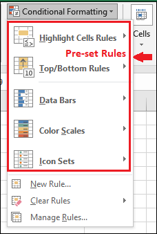

And Microsoft Excel has a vast library of pre-set conditions that users usually want to apply by just using the functions.

Custom conditions

Moreover, the pre-set conditions must meet the criteria we usually want to apply. Microsoft Excel allows us to manipulate the pre-set conditions and define our custom conditions. It means that we can easily create our own set of rules to format the data efficiently.

And from here, we can easily define the custom conditions.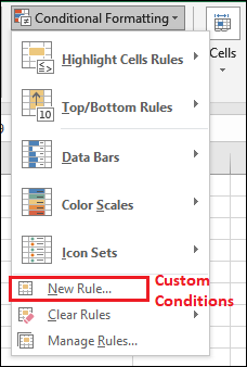

Applying multiple conditions

Sometimes, data requires multiple conditions to be applied to get the exact result that we want. And Microsoft Excel allows us to apply multiple conditions on a single cell. Note that - be aware of the hierarchy and precedence to use them.

Conditional Formatting

Moving further, in this chapter, we will briefly discuss each possible pre-set condition to give an overview to an individual. By just learning their basics, we can easily use them wisely per our needs. When we navigate to the Conditional Formatting option in the Home tab, it also enables several pre-set conditions.

• Highlight Cells Rules
• Top/Bottom Rules
• Data Bars
• Color Scales
• Icon Sets

Highlight Cells Rules

This particular conditional formatting rule allows the users to highlight the cells by just making Use of the pre-set conditions that will meet the specified criteria, and it primarily offers such as conditions to the Microsoft Excel users, such as Greater than, Less than, Between, Equal to, Text that contains Duplicate Values.

These conditions are usually comparison operator conditions.

Top/Bottom Rules

It was well known that this particular conditional formatting primarily contains the top or bottom rules to format the cell data by just highlighting the cells, as it was usually used to highlight the cells from the top or the bottom of the column as well, like top 10 cells or bottom 5 cells.

Top or Bottom rules contain such pre-set conditions, Top 10 items, Bottom 10 items, Top 10%, Bottom 10%, Above Average, and Below Average.

Data Bars

And the Data bars are the colored bars applied to the Microsoft Excel data that represent the value of a cell. These data bars are different than the above two conditional formatting. And they are used to clearly show the higher or the low status of the data contained in the cells.

"Higher the value, longer the bar. Similarly, the Lower the value, the shorter the bar."

1. Data bars are the graphical representation of data. Or that graphical way to show the data.
2. Moreover, the respective Data Bars usually help Microsoft Excel users to show the clear status based on overall data by just highlighting the cells with a color according to the high and low values in the cell effectively.
3. And we need to remember that the data bars only apply to the numeric data type. On String data, these are worthless.
4. Conditional formatting offers several colors to use in Data bars representation.

With the help of an example, we will discuss later how data bars work.

Color Scale

Now in the conditional formatting, a color scale is applied to a range of cells. And the color indicates where each cell value falls within the cell range. In Microsoft Excel, conditional formatting offers twelve color scales to represent the data.
This color scale conditional formatting applies only to numeric values in an Excel worksheet.

Icon Sets

And in Microsoft Excel, we can easily represent the cell's data through the different icon sets. Conditional formatting contains several types of icon sets, such as Directional, Shapes, Indicators, and Ratings.

• For example: By just making Use of the directional icon set, the particular amount of the data can be easily represented in three ways that are none other than high, low, and average values in a column, respectively.

These icon sets only attach with the numeric values in an Excel worksheet, not with String data.

Highlight the cells

We will take an example to highlight the cells by just putting certain conditions in a column.

• For example: Highlight all the cells with data greater than a value (specified by us for the conditional formatting).

And we need to follow below mentioned steps very carefully:

Step 1: First of all, we must select a range of the cells in our Microsoft Excel sheet, e.g., B2 to B8.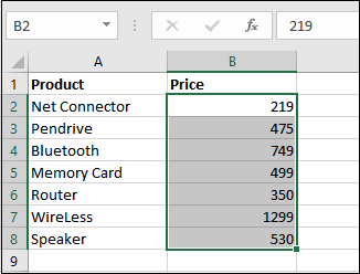

Step 2: Afterward, we need to go to the Conditional Formatting, which is present inside the Home tab, and then click on it.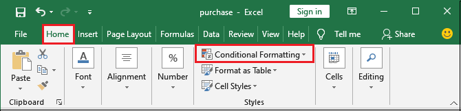

Step 3: Now, in this step, we need to hover the mouse to Highlight Cells Rules in the dropdown list and then will click on the Greater than condition rule as well.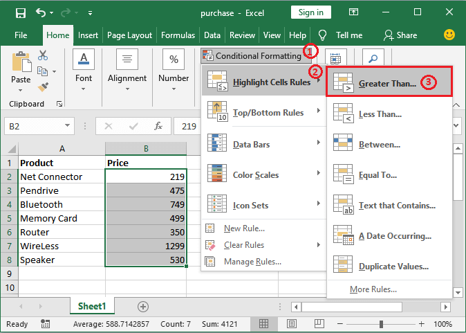

And similarly, we can easily choose any other conditions from here and operate accordingly.

Step 4: In this step, we need to specify a value with which we want to check all the selected values. And here we have entered 65 as well.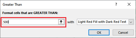

Step 5: We also need to specify the color to highlight the greater values, and then after, we need to press the OK button respectively.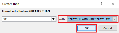

Step 6: In this step, we need to click on the "Ok" option, as clearly depicted in the screenshot below; all the values greater than 65 are highlighted in yellow.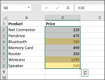

Step 7: And then we need to change the B5 cell value to greater than 500 and will press the Enter key from our keyboard as well.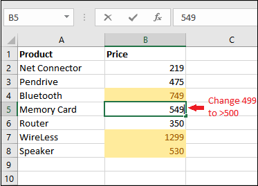

Step 8: Now, in this step, we will see that the cell color is changed to Yellow automatically, and then the cell is highlighted respectively.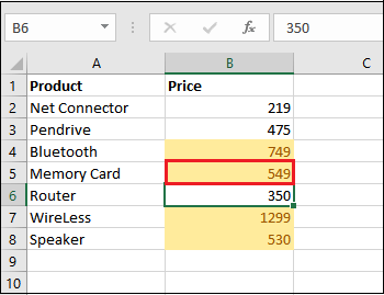

Clear conditional formatting

It was well known that the Microsoft Excel, users can clear all formatting applied to the cells in an Excel spreadsheet at once. And Microsoft Excel allows us to clear the conditional formatting from the worksheet or the selected cells (specific cells). Let us now see both methods, which are mentioned below -

1. Clear formatting from the entire worksheet
Now in the Home tab, we need to go to the Conditional formatting > Clear Rules > Clear Rules from Entire Worksheet.
It will then clear all the pre-set and custom condition rules from the worksheet.

• For example,

Step 1: First, we need to select all the respective cells to clear the formatting from an entire worksheet, and then we need to follow the step to clear the formatting rule for the entire worksheet.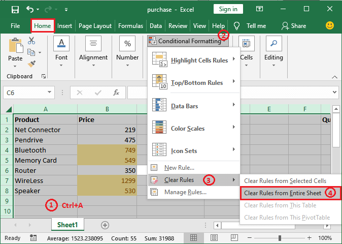

Step 2: By just clicking on the Clear Rules from the entire worksheet, all formatting will be removed from the entire worksheet. Look at the screenshot below respectively:

In this section, we can easily see that the formatting is removed from the entire worksheet (all cells).

2. Clear formatting from selected cells

In addition, we can also clear the conditional formatting from the selected range of cells. And the steps are almost the same as those used in the above part.

In the respective Home tab, we must go to the Conditional formatting > Clear Rules > Clear Rules from Selected Cells.

• For example:

Step 1: First of all, we are required to select the range from B2 to B7 but leave the last one, i.e., B8 cell, and to use the clear formatting rule for the selected cells as well.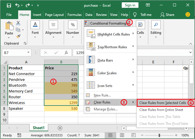

Step 2: Now, by clicking on the Clear Rules from Selected Cells, formatting will be removed only from the selected cells. See the screenshot below: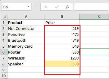

We can all see that the formatting has been only removed from the selected cell, not from all.

Apply the top/bottom rule and highlight the cells.

Conditional formatting enables six pre-set top/bottom rules to highlight the cells. It allows the respective users to highlight the cells from the top or bottom of the column, like top 10 cells or bottom 5 cells, etc.

Top/Bottom rules contain such pre-set conditions, Top 10 items, Bottom 10 items, Top 10%, Bottom 10%, Above Average, and Below Average.

Now we will be seeing out the below-mentioned steps to see how top/bottom rules apply on a column respectively:

Step 1: First, we must select a column (range of cells) and then go to the Conditional Formatting, which is present just inside the Home tab respectively.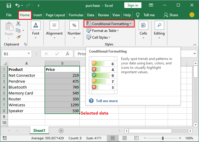

Step 2: Now, in this step, we are required to click on the respective Conditional Formatting option, then will navigate to the Top/Bottom Rules in the list, and will proceed further by choosing one of the Rules from here.

And here in this, we have chosen Above Average to highlight the values which are above average as well.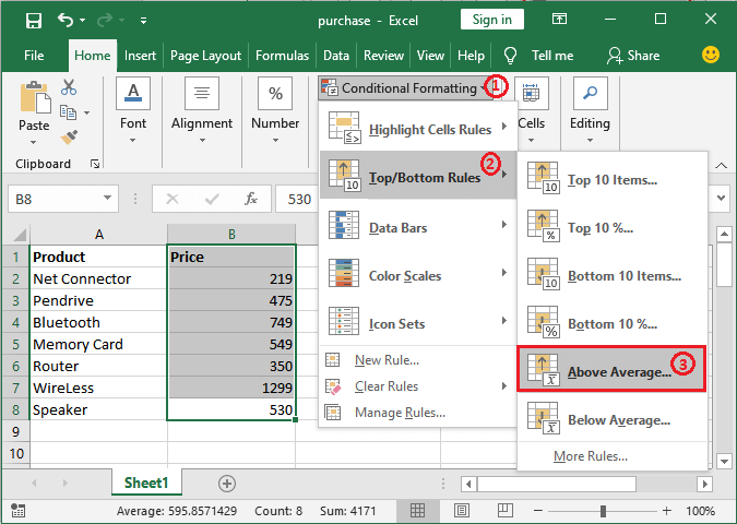

Step 3: Now, in this step, we need to set a color to format the color of the cell and click the OK button.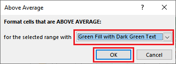

Step 4: Now let us see that all the values above the column's Average are also highlighted.

Applying the data bars to the data

It was well known that the respective "Conditional Formatting" basically consists of the data bars as well, and we can easily use these particular data bars on the numeric data in a given column to represent the value of the cells graphically.
And now, we will be seeing out the steps with which we can effectively achieve the above:

Step 1: First of all, we are required to select or choose a particular column (range of the cells), and then we need to go to the"Conditional Formatting," which is effectively present just inside the "Home Tab" as well.

Step 2: We are required to click on this "Conditional formatting" option and then will navigate to the Data Bars in the given list, then will choose one of the following Data Bars from here.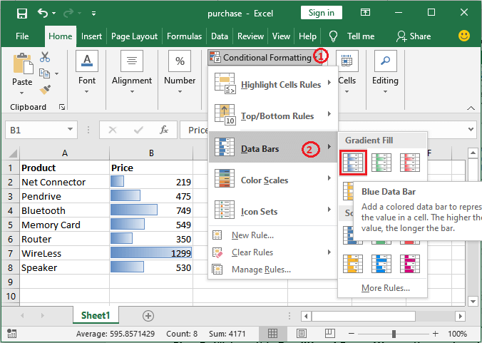

Step 3: Now, in this step, we can see each cell of the respective column is represented by the bar as well.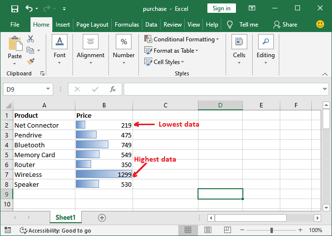
"Higher the value, longer the bar. Similarly, the lower the value, the shorter the bar."

Applying the color scale to data

Now the "Conditional Formatting" primarily consists of several color scales. And we can easily use these color scales only on the numeric data in a given column to represent the value of the cells graphically. And the color indicates where each cell value falls within the cell range.

Let us see the below-mentioned steps on how it could be done and how data is represented respectively:

Step 1: Firstly, we must select two or more columns (range of cells) containing the numeric data, and then we need to go to the Conditional Formatting inside the Home tab respectively.

Step 2: We need to click on this Conditional Formatting option and navigate to the Color Scales in the list; then, we will choose any Color Scales from here.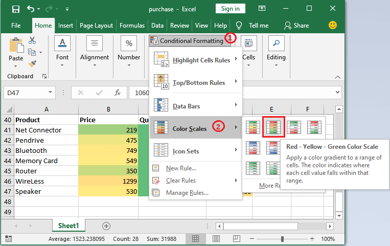

Step 3: After that, we can easily see that the numeric data of the selected column is represented by the color scale respectively.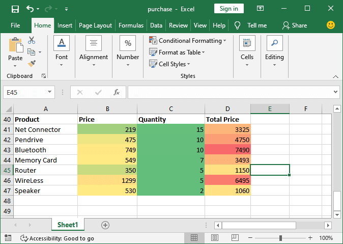

Moreover, we note that the respective color scale can only be applied to the numeric data and not the strings.

Applying icon sets to data.

And in Microsoft Excel, the "conditional formatting" usually offers four types of icon sets, which are none other than the following ones:

1. Directional.
2. Shapes.
3. Indicators.
4. Ratings.
   We can effectively use these sets of icons on the various numeric data in a given column for representing the cell values in a column or the range of the cells. And in this, we will be describing the directional icon set.

Following are the primary steps that can be used to achieve the icon sets with the cell data and effectively represent them:

Step 1: First, we need to select the column (range of the cells) that contains numeric data, and then we must go to the Conditional Formatting that is present just inside the Home tab respectively.

Step 2: Now, in this step, from the "conditional formatting" option list, we will be then clicking on the Icon Sets. And when we click on it, we will get different icon sets, from which we will choose any of them, whichever we want per our needs.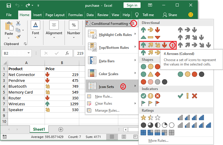

Step 3: Now, we will see that the icon set is primarily attached with cell values and representing them with an arrow, respectively.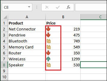

Define custom conditions

It was well known that, in Microsoft Excel, the respective conditional formatting offers pre-set conditions and allows particular users to define their custom rules or conditions. Now in the "Home tab," we must go to Conditional Formatting > New Rule respectively.

From here, we can easily set up particular custom rules. Let us take an example to understand better as well.

• For example, Row to row comparison of the two columns and the highlighting of the cell if matches are found.

Step 1: First of all, we need to have this dataset for comparison and select a row in which we want to check whether the values are the same.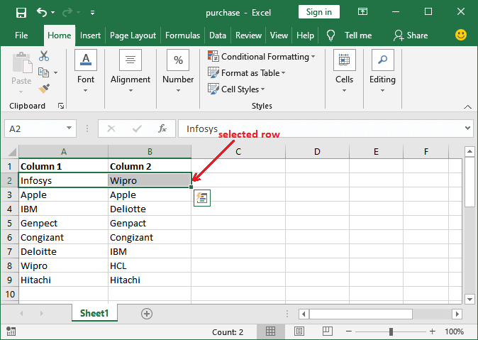

Here, we can easily compare simple data only by just seeing the data. But for complex data, it takes work to match the values respectively.

Step 2: Now, in this step, just under the Home tab, we are required to go to the Conditional Formatting > New Rule.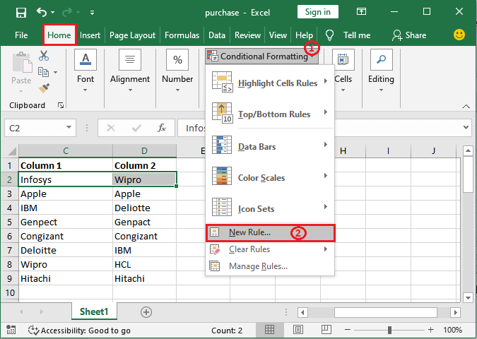

Step 3: Here, we must click the Use a formula to determine which cell to format from the rule type list.

Step 4: Here, inside the formula field, we need to specify the cells which we want to compare in the following format, e.g., =$A2=$B2 for the second Row, respectively.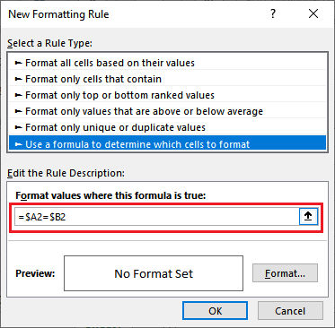

Step 5: In the end, we are required to specify the format for matched cell by just clicking on the Format button, and then we need to see the preview inside the Preview box respectively.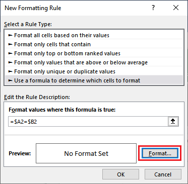

Step 6: Here, we can navigate to the Fill tab, and then we will choose a background color to highlight the matches and click on the OK button.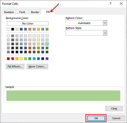

Step 7: And then we need to see the preview inside the preview section and will see how the Row will look if the match is found. After that, we need to finalize everything, and we will click on the OK button to save the changes as well.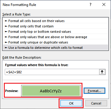

Step 8: Now, we will see that the respective selected Row has not been highlighted because the A2 and B2 cells do not contain the same values.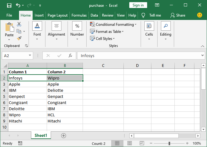

Step 9: By following the same steps, we can easily compare the next Row of data. See that everything is set up successfully. Now, we will click the OK button to get the result.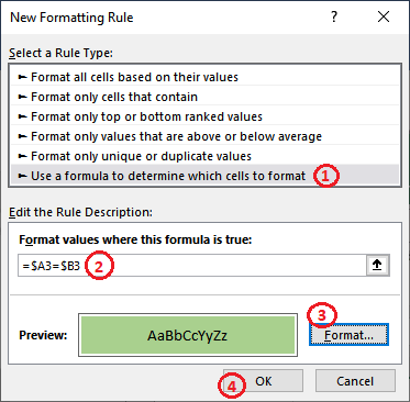

Step 10: We will look at the following screenshot, that the 3^rd Row has been highlighted because it gets the same data in both columns.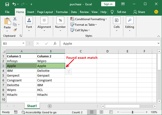

Step 11: Similarly, we will check for all the rows one by one. And see the Excel worksheet after comparing both columns. That Row having the same data in both columns has been highlighted and remains as it is.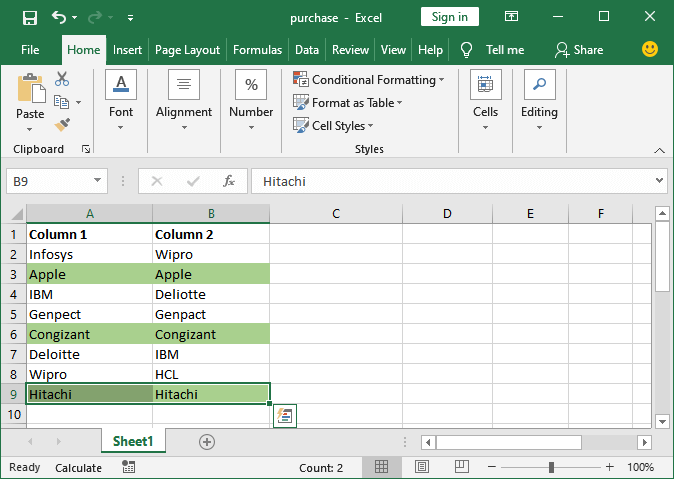

It will highlight the entire matching data row in the format we previously chose. Through this, we can easily define the custom conditions in conditional formatting.