Merging Duplicates in ExcelIn Excel, merging duplicate rows refers to combining entries from different worksheets to improve organization and presentation. We frequently need to combine duplicate rows in Excel when working with it at home, at work, in retail stores, or corporate settings. Various easy-to-use and efficient methods exist to integrate duplicate worksheet rows and total the results in Excel. We will now illustrate and provide appropriate examples for five of them. Let's say we have an Excel worksheet with a data set that includes the sales information of multiple sales representatives. To ensure that each sales representative and his total sales are listed in the table only once, we must combine the data sets. 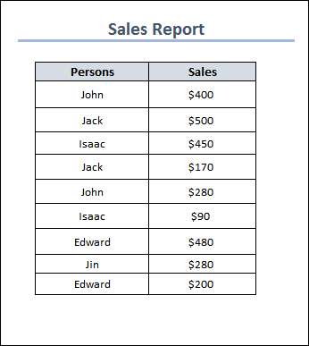
To combine our sample data, we will demonstrate five popular techniques for combining duplicate rows. You will understand how to combine duplicate rows in Excel after reading this tutorial by using:
1. Using Excel's Consolidate Option to Combine Duplicate RowsInformation from several rows, worksheets, or workbooks can be consolidated into one location using the Consolidate option. It assists you in compiling the data from your data table's various locations. We'll examine how this tool helps us resolve our issues step by step. On the right side, we created a table to collect the consolidated data. 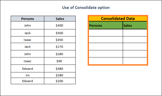
Procedure:
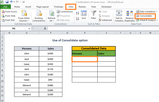
Then, the Consolidate dialog will launch.
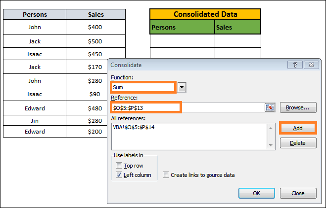
Our chosen Range will then show up within the entire references box. 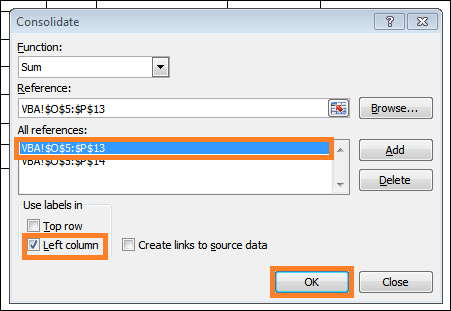
Upon completion, you will receive a distinct roster of sales representatives plus an account summary derived from your original data set. 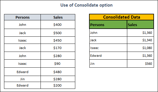
2. Utilizing Subtotal FeatureHere, the sales values for the duplicate Persons will be combined using the Subtotal feature. 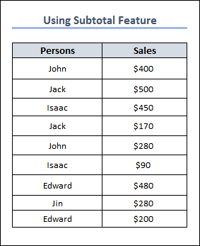
Procedure: We must first sort the names alphabetically to keep the duplicate titles together.
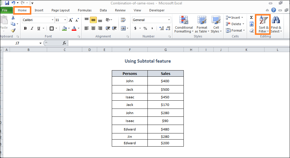
The Sort dialogue box is going to open later.
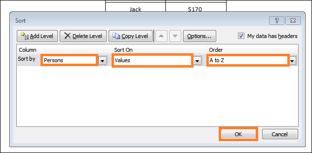
The following order was later created by placing the Sales values in relation to their respective Persons. 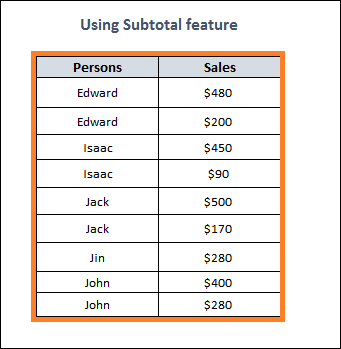
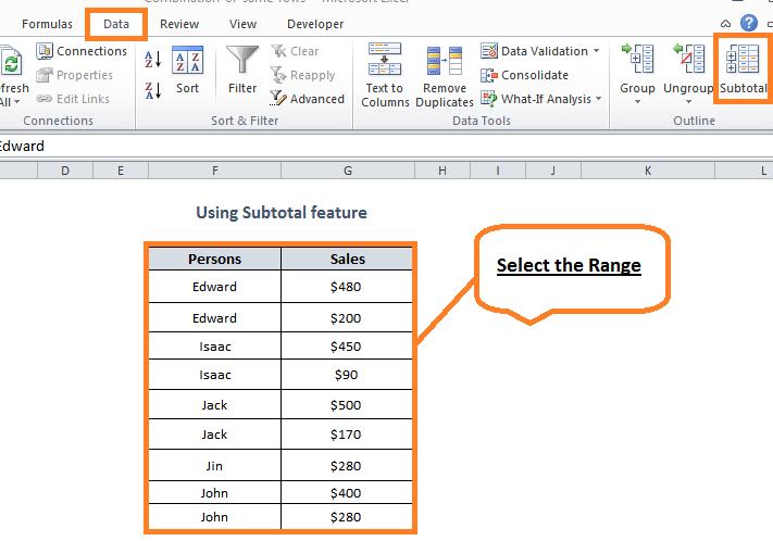
A subtotal dialog box will appear after that.
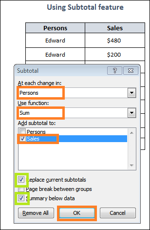
Every Persons's sales will subsequently be combined and totalled after being grouped. 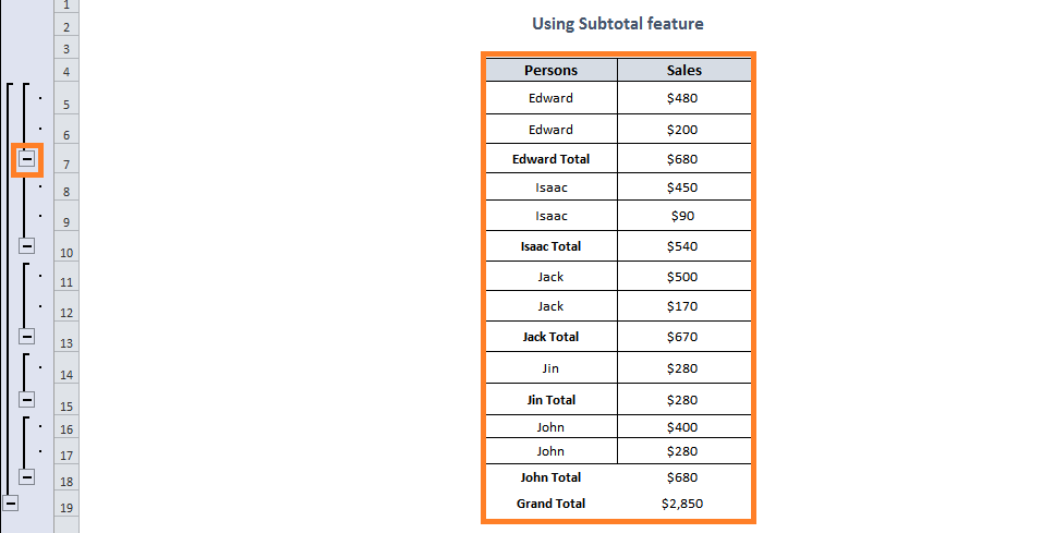
Thus, it's evident that Edward's duplicate rows have been combined in this instance. 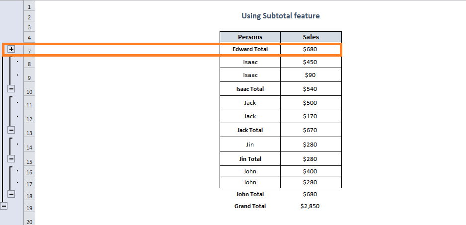
We have completed this task for other representatives of sales in a similar manner. 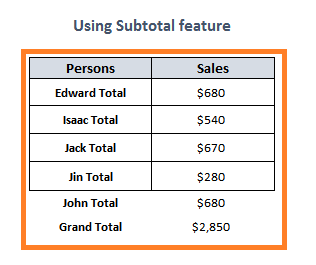
The final two rows can have borders added to them. 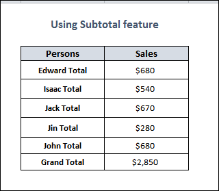
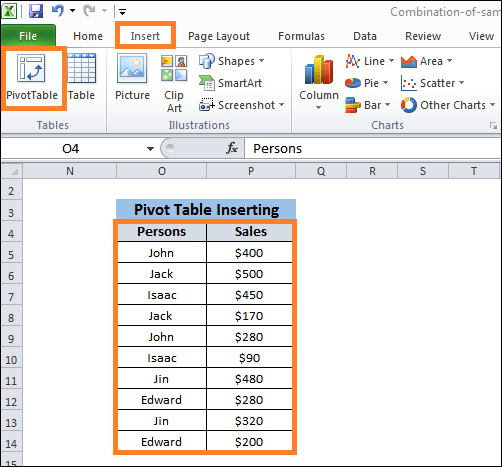
3. Using a Pivot Table in Excel to Combine Duplicate RowsA pivot table is one of the best tools for aggregating, combining, and examining data in Microsoft Excel. We'll demonstrate how to use this tool to merge duplicate rows and accomplish our goals using this method. 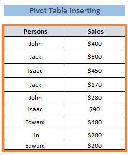
Procedure:
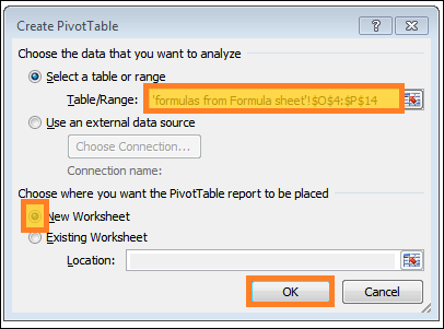
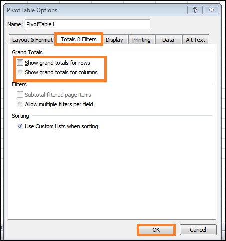
It will open the Create PivotTable dialog box. You can see that the Table/Range field now displays your selected range.
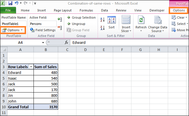
Consequently, you will be redirected to a new sheet with the PivotTable on the left and the PivotTable Fields on the right. 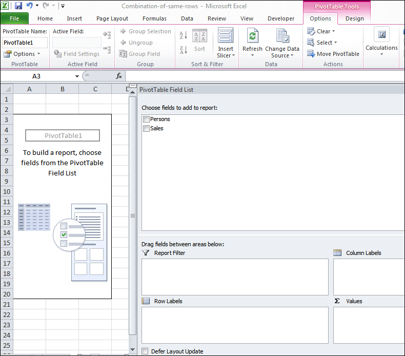
The Pivot Table will then show up on the left. 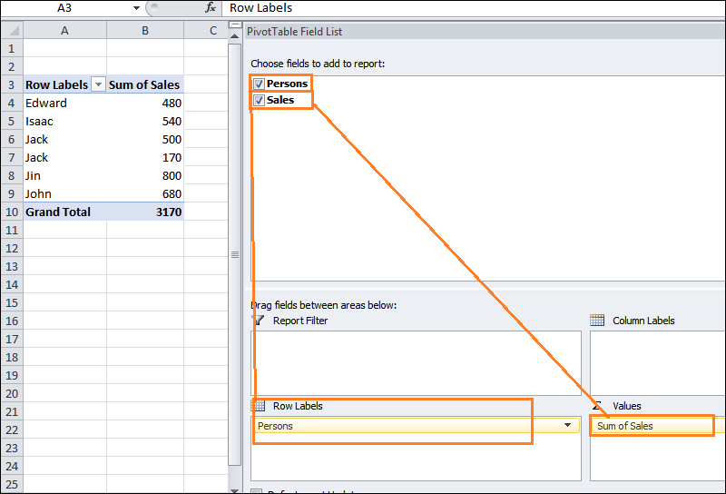
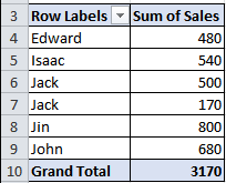
The following table will show up, with the rows for duplicate people merged. 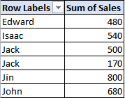
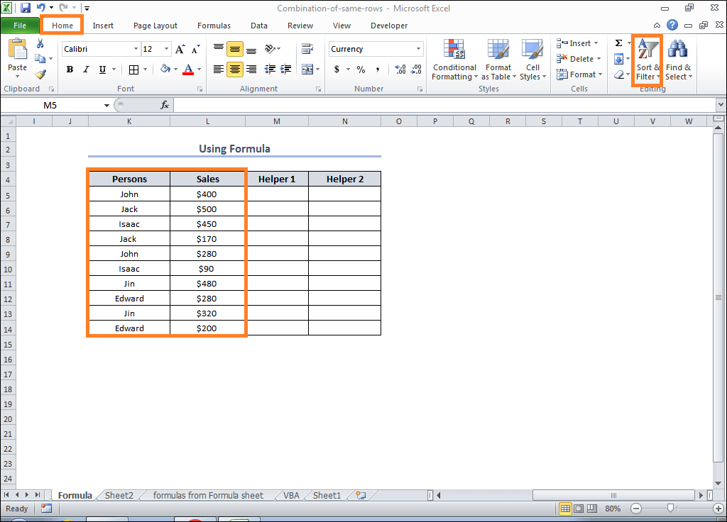
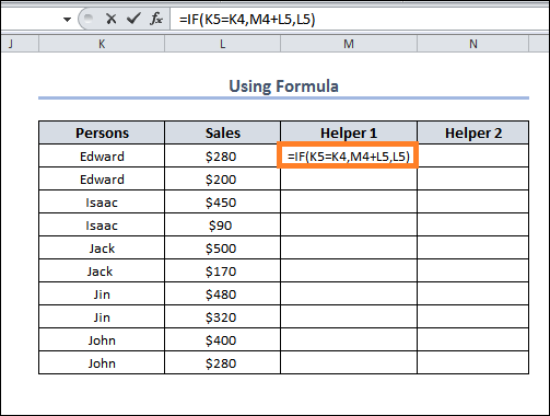
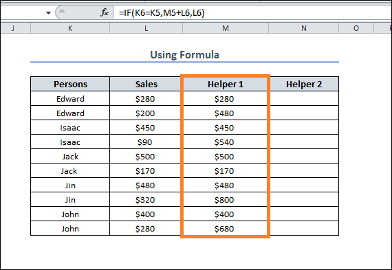
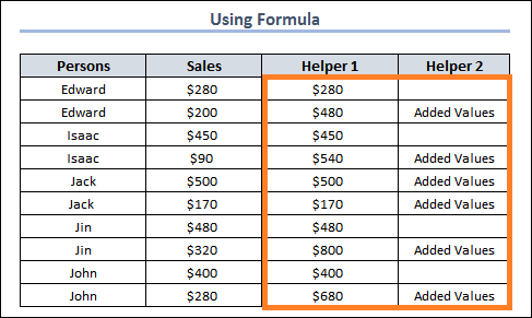
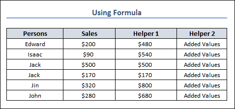
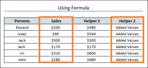
4. Using the IF Function in Excel to Combine Duplicate RowsTo add the sales values for the duplicate names, we will first use the IF function in this section to merge the duplicates of the Persons column. Helper 1 and 2 are the two columns we added for this purpose. 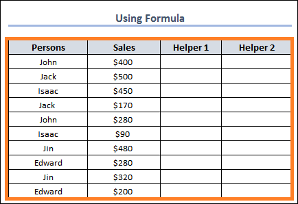
Procedure:
The Sort dialog box is going to appear afterwards.
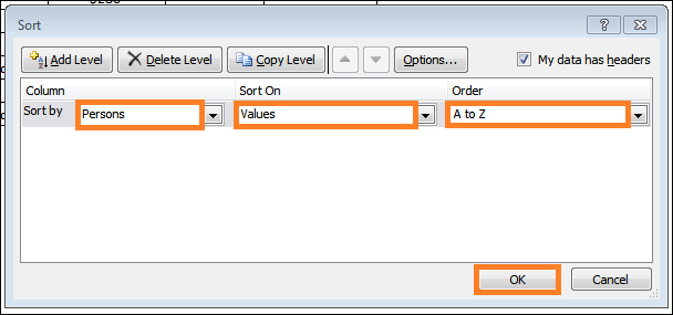
The following order has since been created for the sales values and the corresponding Persons. 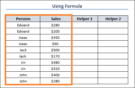
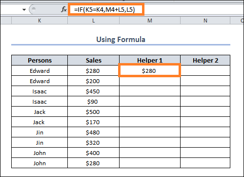
Formula Explanation
Formula Explanation
The Filling Handle tool can be dragged to get the remaining values. 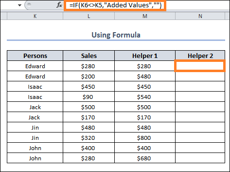
You will then receive Added Values of the rows that are duplicates. 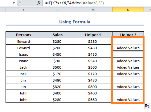
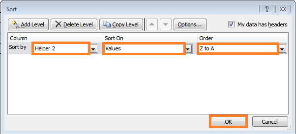
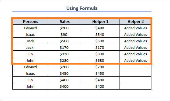
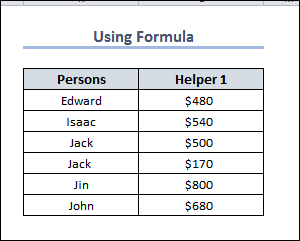
We will remove the formulas and retain the values in the following table since we need to sort it according to the final column.
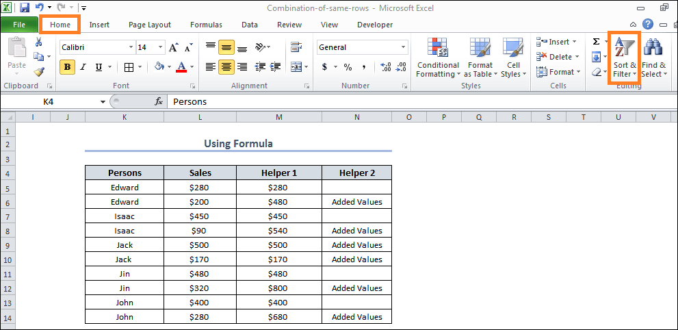
The Dialog box for Sorting will open later.
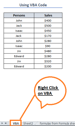
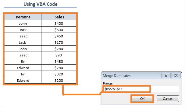
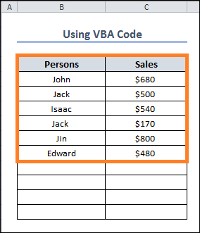
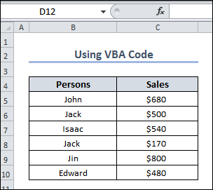
5. Using a VBA Code to Combine DuplicateAdditionally, the VBA codes facilitate the worksheet's merging of duplicate rows. We'll walk you through the process of using VBA code in MS Excel to combine duplicate rows. 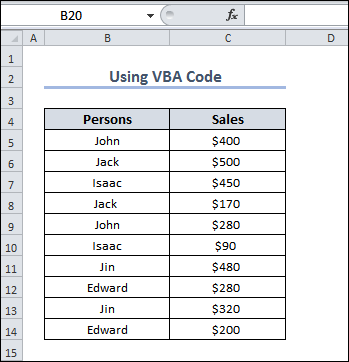
Procedure:
Code:In this case, whole_list is declared as Range & cell_V, modified_list is displayed as Variants, and On Error Resume Next is used for ignoring the error and carrying out the code execution into the next cell. The UBOUND function determines the size of the array, and the FOR loop applies for a range of rows beginning with Sales_rep = 1. 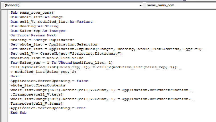
Next TopicExcel 365
|
 For Videos Join Our Youtube Channel: Join Now
Feedback
- Send your Feedback to [email protected]
Help Others, Please Share


