Correlation in Microsoft Excel: coefficient, matrix, and graph

In Microsoft Excel, Correlation is considered to be one of the simplest as well as the most basic calculations (statistics) that we can perform. Though it is very simple to use, it is useful in understanding the relations between two or more variables that are used in the Excel sheet for calculation.

And besides all this, Microsoft Excel primarily provides all the necessary tools to run out the correlation analysis. In these tutorials, we will be discovering the below-mentioned topics respectively:

1. What do you mean by Correlation- the basic in Microsoft Excel?
2. What is meant by Correlation coefficient in Microsoft Excel?
3. What do you mean by Pearson correlation in Microsoft Excel?
4. Correlation Formula in Microsoft Excel?
5. How to find out the correlation coefficient in Microsoft Excel?
6. What are the things which need to be remembered by an individual In Excel?

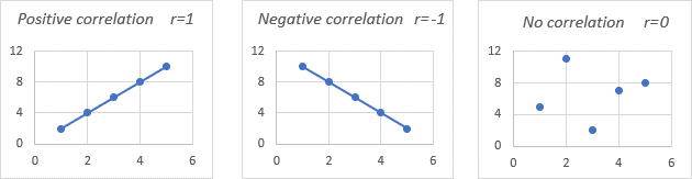
What do you mean by the term correlation in Microsoft Excel?

Correlation in Microsoft Excel is a measure that is used to describe the strength as well as the direction of a relationship that exists between the two variables effectively.

Furthermore, the Correlation functions are the most commonly used in statistics, economics, and the social sciences in order to create budgets, planning of business, etc.

And the efficient methods that are used in Microsoft Excel is to study how closely the variables are related and are termed as correlation analysis.

Now we will be seeing a couple of examples that are related to the strong Correlation:

1. The number of calories an individual takes and their weight (positive Correlation).
2. The temperature outside (negative Correlation)

And here the examples of data that have weak or zero amount of Correlation:

1. An individual pet's name and favorite food intake
2. Height of an individual and the color of their hair.

And the most important thing that needs to be remembered about Correlation is that it is only used to show how closely the two variables are related and does not imply any causation.

The fact that changes in one variable are closely associated with changes in the other variable does not mean that one of the respective variables causes the different variables to get change effectively.

What is meant by the term Correlation coefficient in Microsoft Excel?

In Microsoft Excel, the correlation coefficient (r) is the numerical measure of the degree of association between the two continuous variables.

And the given coefficient value usually lies in between of -1 and 1, and this could be effectively used for the purpose of measuring out the strength as well as the direction of the linear relationship lies in between of the variables.

1) Strength

We can assume that, larger the absolute value of the coefficient stronger the relationship will get exits:

• The particular extreme values of -1 and 1 will be indicating out a perfect linear relationship when the data points fall on a single given line.
• And a coefficient of 0 indicates that there is no linear relationship that will be exiting in between the variables, and this is because we need to go with the two sets of random numbers.
• Moreover, the values between 0 and +1/-1 usually represent a scale of weak, moderate, as well as strong relationships.

2) Direction

In Microsoft Excel, the coefficient sign that is plus or minus used to indicate the direction of the relationship respectively.

• Positive coefficients: The positive coefficient represents the direct Correlation and produces an upward slope on a given graph - if one of the variables increases, others will also increase.
• Negative coefficients: The negative Correlation is used to represent the inverse Correlation and hence produce a downward slope on a given graph - as if one variable moves on increasing, the other variable tends to be in the decreasing direction.

And now, in order to get a better insight into the above-used function, we will be looking at the below-mentioned graph as well:

1. A coefficient of 1 means a perfect positive relationship; one variable increases, and the other increases proportionally.
2. And a coefficient of -1 means that it is a perfect negative relationship - as in this, one of the variables tends to be in the increasing direction while the other decreases.
3. A coefficient of 0 means that there exists no relationship between the two variables:

What do you mean by Pearson correlation in Microsoft Excel?

We all know that statistics measure several types of Correlation, which depend on the kind of data with which we work.

The Pearson Correlation in Microsoft Excel stands for the Pearson Product Moment Correlation(PPMC) that is used for the purpose of evaluating linear relationships between the given data when a change in one variable is associated with a proportional change in the other variable respectively.

In simple terminology, the Pearson Correlation also answers the basic question: Can the data be represented on a line?

In statistics, it is the most popular correlation type. If we are dealing with a "correlation coefficient" without further qualification, it is likely to be only Pearson.

And the most commonly used formula that can be effectively used to find the Pearson correlation coefficient in Microsoft Excel is also termed to be Pearson's R: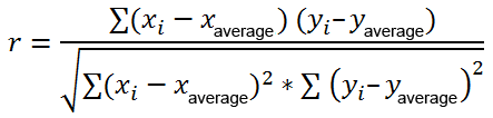

And at the same time, we may come across two other formulas that can be used to calculate the sample correlation coefficient (r) and the population correlation coefficient (?), respectively.

How can one find Pearson correlation in Microsoft Excel?

Calculating the Pearson correlation coefficient by making use of the hand involves much math. And luckily, Microsoft Excel has made out things much simple. Depending on our data set and our respective goal, we are free to use one of the following techniques as well:

1. First, find the Pearson correlation coefficient with the help of the CORRELATION FUNCTION.
2. And one should need to make a correlation matrix by just performing the Data Analysis on the given excel sheet.
3. Moreover, we need to find the multiple correlation coefficients by using the formula.
4. And then, we will be plotting a correlation graph to get the data relationships in visual representation.

CORRELATION Formula in Microsoft Excel

The correlation formula that is primarily used in Microsoft Excel is as follows:

Formula: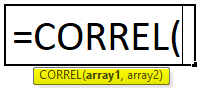

Which the,

1. Array 1: Array 1 is an independent variable used in the correlation formula and is entered as a cell reference or the range of values.
2. Array2: Array 2 is considered a dependent variable used in the correlation formula and could be entered as a second cell reference or the range of values.

• And a coefficient of zero indicates that there is no discernable relationship between the variables' fluctuations.
• It is the most commonly used function to calculate the correlation coefficient for the given two sets of values or the variables, i.e., the Correlation between particular stocks.

How to make use of the CORRELATION Function in Microsoft Excel?

The CORRELATION Function in Microsoft Excel is primarily considered as simple to use function. Now after that we will be seeing how one can make use of the CORRELATION function in Excel with the help of the various examples.

# Example 1: For a Set of Positive Variables or Dataset in Excel sheet

With the help of the Correlation function, we are required to find out the correlation coefficient that is effectively exiting in between of the two datasets or the variables as well.

The below table contains the two variables, one in column X and the other one in column Y, in which both the datasets include positive values: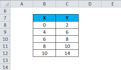

Step 1: Now we will apply the Correlation function in the cell "C14". And then, we will select the cell "C14" in which the function needs to be used.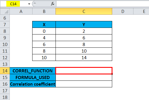

Step 2: Now in these step, we will be clicking on the insert function button (fx), that is present just under the formula toolbar, and soon after clicking the dialog box will get appears on the screen; then we will typing out the keyword that is "CORREL" in the search for a function box, the CORREL function will get appears in the select function box. We will be double-click on the CORREL function respectively.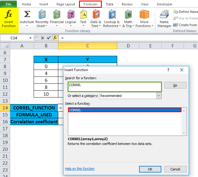

Step 3: A dialog will appears on the screen in which we need to fill out the arguments for the CORREL function to carry out.

Now for the Array1 argument, we will be clicking just inside the cell B8 and see the cell selected; then, we will determine the cells until B12. So that column range will be chosen from cell B8 to cell B12 respectively.

Now for the Array2 argument, we will be then clicking inside the cell C8 and will see that the cell gets selected; then after that we will be determining the cells until cell "C12". So that column range will be chosen from cell C8 to cell C12.

i.e. =CORREL (B8:B12, C8:C12) which will gets appear in cell C14.

And after entering both array arguments, we will click on the "ok" option.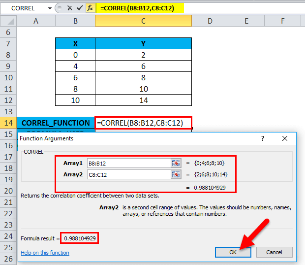

Step 4: After that, it will return the output as 0.988104929, where the Correlation coefficient between the two datasets or the variables is 0.98.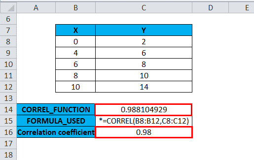

The Graphical representation can also be done using the line chart, which is present just under chart options.

We are having two variables that are X and Y, where one is plotted on the particular X-axis and the other on the Y-axis as well.

For this, we will be selecting the table range excluding the header X as well as the Y that is from cell B8 to cell C12 respectively: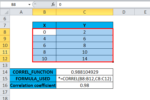

After that, we will click on the Insert tab, which is present just under the line options, and select the first one in the line chart option.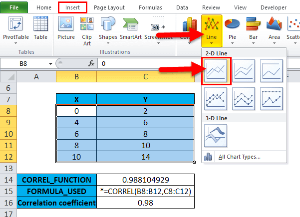

As soon we perform all the above steps, it will give the specific chart following the value mentioned: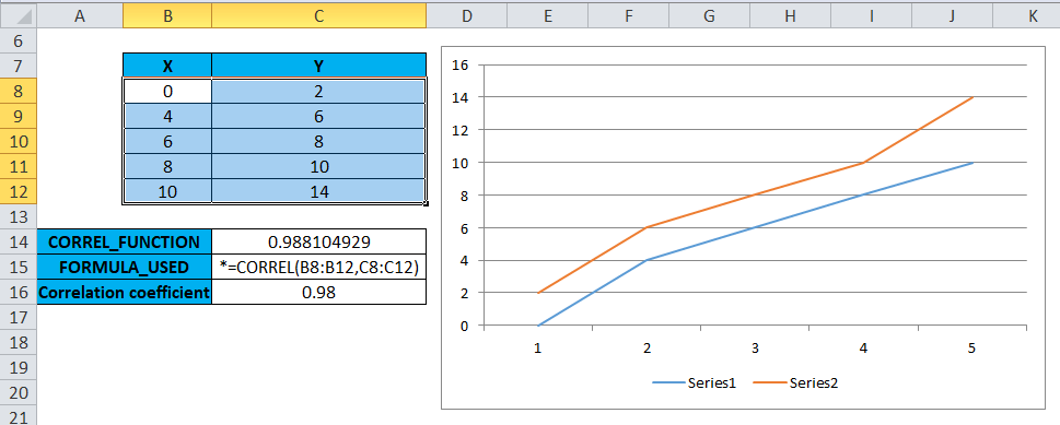

And the chart elements such as legend series (X, Y) axis title (X and Y axis), chart title (POSITIVE CORRELATION) as well as the data label (Values) need to be updated in the chart as well.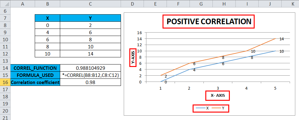

# Example 2: For a Dataset Containing Positive & Negative Values in Microsoft Excel

With the help of the Correlation function, we need to find the correlation coefficient between the two datasets or the variables.

In the below-mentioned example, we have used two variables; one is primarily represented in column x and the other in column Y. The column X datasets usually contain positive values, and the column Y datasets contain negative ones.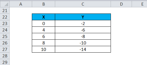

Step 1: Now, we will move on by applying the Correlation function in the particular cell, "C29". And we will be selecting the cell "C29," in which the Correlation function needs to be applied.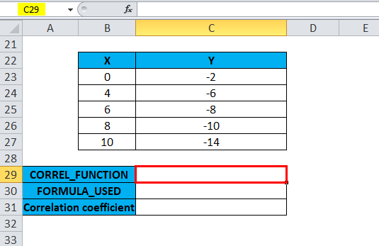

Step 2: And now after that we will be clicking on the insert function button (fx) that is present just under the formula toolbar; a dialog box will get appear on the screen, and we will then typing the keyword "CORREL" in the search for a function box, and the CORREL function will calls will get appear in the select function box. After that, we will be double clicking on the CORREL function respectively.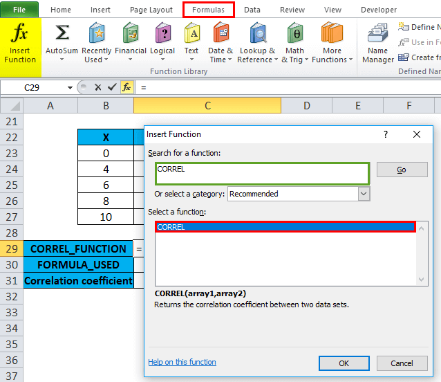

Step 3: A dialog box will appear on the screen where we need to fill out the required arguments for the CORREL: =CORREL (array1, array2).

And for the given Array1 argument, we will be then clicking inside cell B23, and we will get encountered with the selected cell; after that we will be selecting the cells till B27. So that column range will be chosen from cell B23 to cell B27.

Similarly, for the Array2 argument, we will click inside cell C23, encounter the selected cell, and select the cells till C27. So that column range will get selected effectively, from cell C23 to cell C27.

And =CORREL (B23:B27, C23:C27) will appear in cell C29.

And after entering both array arguments, we will click on the "ok" option.

Step 4: After that, it will return the output as: -0.988104929, whereas the Correlation coefficient between the two datasets is -0.98, respectively.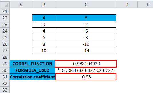

Similar to the above example, it can also be represented graphically by using a line chart which is present just under chart options.

We are having two variables, X and Y, in which one is plotted on the respective X-axis and the other on the Y-axis.

Moreover, we can see the negative Correlation, i.e., Variables X and Y values are negatively correlated (Negative linear relationship). In this case, y moves on decreasing when x goes on increasing.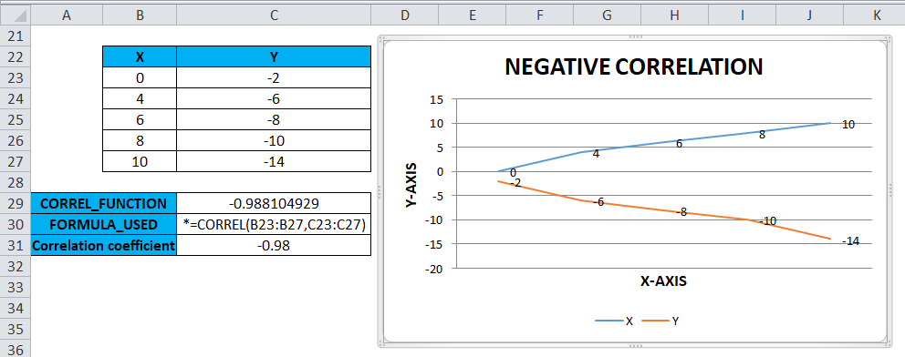

What important things need to be remembered while using the Correlation function in Microsoft Excel?

The important points, as well as things that are required to be remembered by an individual while dealing with the Correlation Function in Microsoft Excel, are as follows:

1. If Array1 and Array2 have a different number of data points or if the supplied arrays are of different lengths. Then the CORREL function results in or returns the #N/A error value respectively.
2. And the function will be returning the #DIV/0! Error value if the argument array1 or array2 contains non-numeric data like text, logical values, or blank cells, respectively.
3. And the other most important method that can be used to calculate the correlation coefficient is through the Data analysis option.
   Besides all these in the respective excel toolbar, the data analysis tab is selected just under the data ribbon; and once we will be clicking on the given data analysis, a Data analysis popup will get appears on our screen; in that, we are required to select Correlation in order to calculate the correlation coefficient for the given datasets or the variables efficiently.
4. And it is an in-build Analysis Toolpak Add-in which is present in application add-ins.