Excel tricks

Excel is a powerful tool for storing and manipulating data in tabular form. You can learn basic usage of Excel from any online Excel tutorial. But this will be simple learning. By knowing some Excel tricks, you will become a power user of Excel.

Excel has so many tricks that will help you to make the work easy and fast. If the user work normally with, the process of working will be bit slow. These tricks will help you do the task faster than the usual work process.

In this chapter, we will discuss the ten most useable tricks of Excel that will help the users to fulfill their needs.

Top 10 Excel tricks

We are discussing some most helpful tricks of Excel that will help you to work like a pro. These tricks are -

• Trick 1: Open multiple Excel files in one click
• Trick 2: Shift between different files without mouse
• Trick 3: Select all cells with a single click
• Trick 4: Delete blank rows in Excel faster
• Trick 5: Create shortcuts menu in Excel
• Trick 6: Data validation on Excel data
• Trick 7: Replace data row to column
• Trick 8: Hide data thoroughly
• Trick 9: Autofill
• Trick 10: Add multiple rows or columns at once

Trick 1: Open Excel files in one click

Sometimes, you need to work with multiple Excel files at the same time. You usually open the file one by one, which takes too much time to open each file individually. We have a trick for you to open multiple Excel files in bulk. This trick will save your time and also make the work faster.

Select the Excel files you want to open and press the Enter key. All the selected files will be opened simultaneously.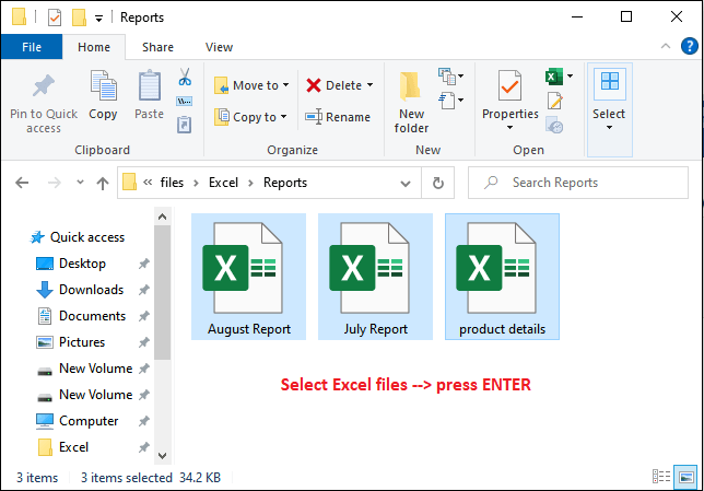

Trick 2: Shift between different worksheets

When you work on multiple Excel files at the same time, it is very annoying to switch between the files with a mouse click.

Excel supports switching between different sheets using the Ctrl+Tab key. It allows the users to switch between different Excel worksheets freely when they work with multiple files.

Trick 3: Select all cells with a single click

You might be wondering that all the text editor has a shortcut key Ctrl+A to select all data then what is different in this trick. Excel offers a unique feature to select the entire worksheet data in one click.

You have seen a triangle shape button on the left corner (between column A and row 1) of your worksheet. This triangle button is actually a select all data shortcut trick of Excel.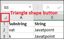

Click this triangle-shaped button to select the entire sheet data.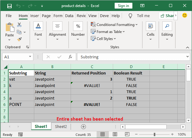

Trick 4: Delete blank rows in one go

In some cases, your Excel sheet may contain some blank rows. You need to delete them to maintain the data accuracy, such as to calculate the average. You don't have to put too much effort; you just have to follow three simple steps described below -

1. To delete the blank rows that consist of between your Excel data, press the F5 function key and go to Special.
2. Here, mark the Blank radio button and click OK. It will select all the blank rows appearing between your Excel data.
3. Now, inside the Home tab, click on Delete option to delete the selected blank rows.

Trick 5: Create shortcuts in Excel

Excel offers three default shortcut options in the Quick Access bar, i.e., Save, Undo, and Redo. When you work on Excel data, you require some options repeatedly. But you need to follow the lengthy steps to reach out to those options in Excel.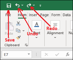

You can customize the Quick Access Toolbar and add the options you want to it. Go to File > More > Options > Quick Access Toolbar. Now, choose the command, which one you would like to quick access toolbar.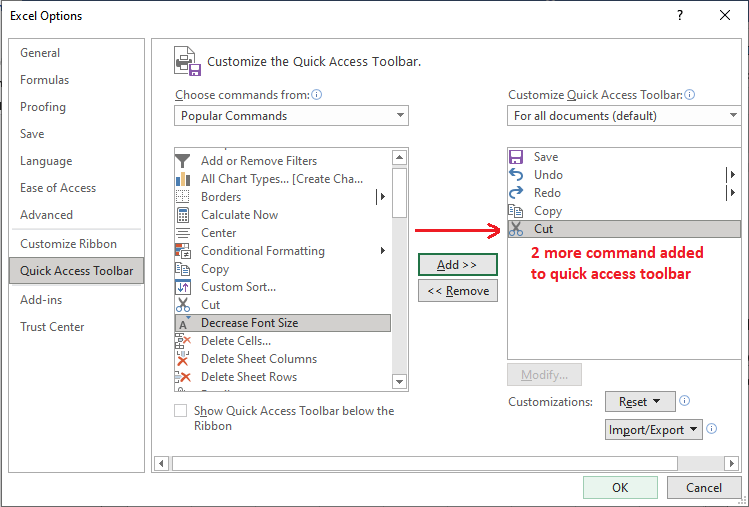

We have added Cut and Copy to the quick access toolbar.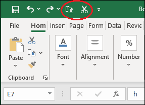

Trick 6: Data validation in Excel

Data validation is one of the most useful features of Excel. It allows the Excel users to put the validations on cells, columns, or rows that restrict the users to put the insufficient value inside them.

For example, You need the employees details for which you have shared an Excel sheet with them to fill details in it. It might be possible that some employees are not aware with some fields and put the invalid data. In that case, data validation will help you to put the data validation on each column along with related column details. So, your employees will not get confused and Excel also does not accept incorrect data type information.

Steps to put Data validation

Go to Data tab > Under the Data Tools section, click on the Data Validation option.

Now, set the validation of any type which one you want to place on your Excel column/cell here.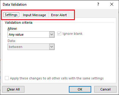

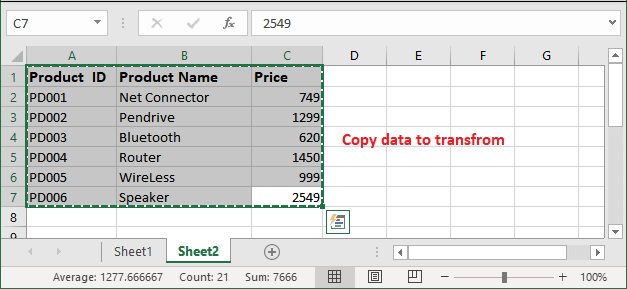
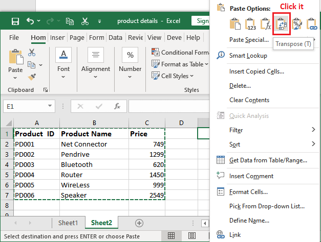
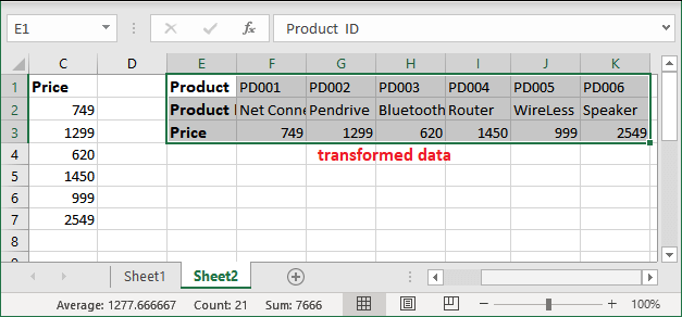
1. Settings tab: In setting tab, define validation.
2. Input Message tab: You can also provide an input message to let the user to type of data being entered. Inside the Input Message tab, provide an input message. This input message will show when the validation cell is selected to enter the data.
3. Error Alert tab: Besides this, you can also provide Error Alert on entering invalid data inside the validated cells. Inside the Error Alert tab, provide an error message.

Trick 7: Replace row to column

Excel allows its users to transform the row data to column and vice versa. In case you need to display the rows data as column, you can follow this trick. Being retyping the whole data to transform it from row to column, use the Excel trick and transpose the data from row to column.

1. Copy the data you want to transpose and go to the blank location where you want to show the transformed data.
   
2. Right-click and select Transpose under Paste Options. This will transform the rows data into columns.
   
3. You will now see that the selected data is transformed from row to column start from column E.
   

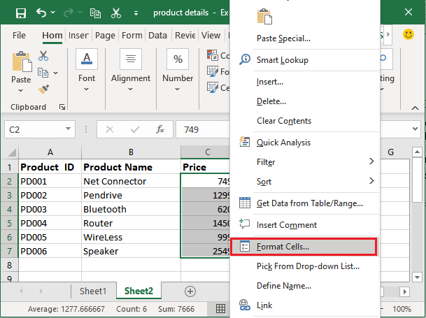
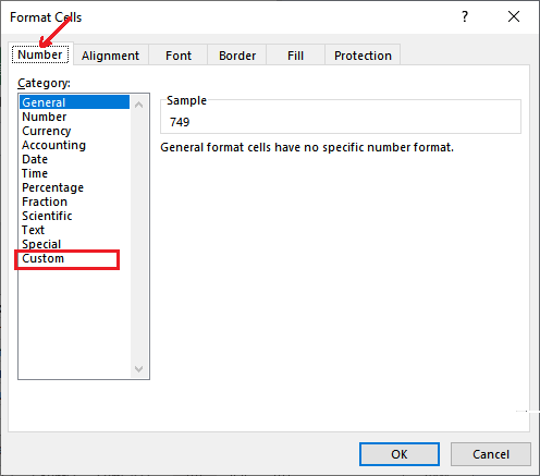
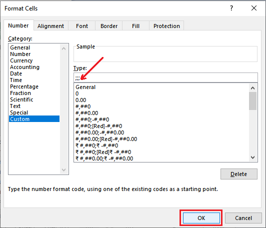
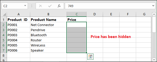
Trick 8: Hide data thoroughly

Almost all users know the traditional way to hide the data in Excel, i.e., right-clicking and select the Hide function. The problem is that - it can be easily recognized if there is only a bit of data. So, to hide the data thoroughly, you can use the Format Cells function.

1. We have the following data. Here, we will hide the price details of the products.
   
2. Select the range of cells to hide. Right-click and choose Format Cells.
   
3. Inside the Number tab, choose Custom.
   
4. Remove pre-defined data inside the Type field and write semicolon like this ;;; and click OK.
   
5. These hidden values are now only found in the preview area (next to the Function button).
   

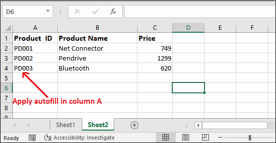
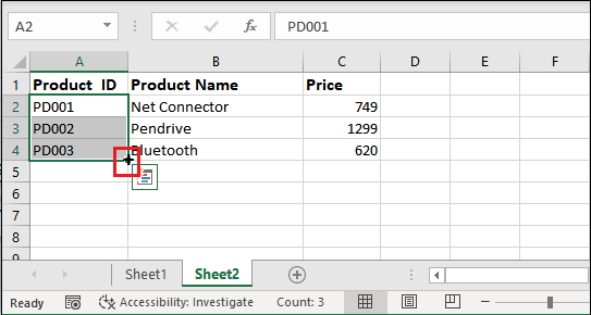
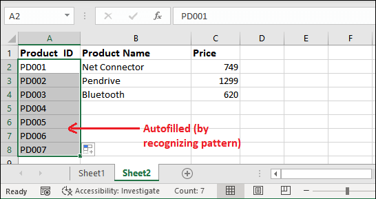
Trick 9: Autofill

Excel autofill feature is a huge time saver, but the users are rarely aware with this feature. When you need to enter the same pattern of data in a column, use the autofill feature of Excel. It recognizes the pattern and fills the data into cells.

It can be string, numeric, alphanumeric, or any type of data. Let's see how to save time by using this feature.

1. Column A is containing alphanumeric data, i.e., Product Id.
   
2. Select the data entered in column A and take the mouse at the bottom right corner of the last selected cell. You will see a + sign there.
   
3. Drag this + sign to below in the column, the data will be automatically filled inside the column by recognizing the pattern.
   

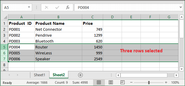
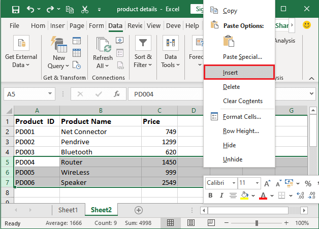
Trick 10: Add multiple rows or columns at once

You have inserted a row/column into your Excel file. What if you need to insert multiple rows or columns? Several times, you need to enter multiple rows or columns in your Excel file. If you follow the usual process to insert a single row or column, it takes time to enter one by one.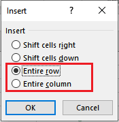

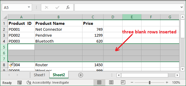
This inserts a single row or column into the Excel sheet at once. We have an Excel trick to insert multiple rows or columns at once.

Insert multiple rows

1. Select the number of rows before which you want to insert the row. For example, we have selected three rows here. So, the three blank rows will be inserted above the selected rows.
   
2. Right-click on the selected row and choose the Insert option in the list.
   
3. You will now see that the three blank rows have been inserted at once.
   

Similarly, you can insert more rows and columns in the same way.