Merge Two columns without losing data

In Excel, data entered by the user is a combination of rows and columns. Based on the requirement, the data present in the worksheet is edited or organized. Sometimes there requires combining rows or columns with working with the data. While merging the respective columns, the data present should be preserved and intact.

Why is there a need to combine the columns?

There are several reasons to combine the data present in the columns. Some of the reasons are listed as follows,

• Similar data: If the data present in the two columns are identical, then combining the respective columns helps to organize or work with the data.
• Formatting: To create a specific format or layout for the data, combining two columns helps to achieve the form of the data.
• To remove duplicates: Merging the column is the quickest way to find and remove duplicates. The column with similar data is easily found and removed by merging the columns.
• Sorting: To sort the data based on the desired order, merging the columns helps to achieve sorting.
• To create labels: To develop clear and appropriate labels or headers for the data, merging the columns can create the brand.

How to combine two columns without losing data?

To combine two columns without losing data, various methods are used. The ways are as follows,

1. Concatenation Function

In Excel, the CONCATENATE function is used to combine two or more text strings into a single cell. The CONCATENATE function is proper when you have data in multiple columns that you must merge into one column.

Syntax:

=CONCATENATE (text1, [text2], [text3],...)

Parameters:

text1 (required): This parameter represents the required text strings you want to concatenate.

text2, and text3 (optional): These parameters represents the optional text strings. You can concatenate up to 255 text strings using this function.

For example, if you have data in columns A and B and you want to concatenate the data in these columns into column C, you can use the following formula:

=CONCATENATE (A1, " ", B1)

This will concatenate the data in cell A1, followed by a space, and then the data in cell B1 into cell C1.

Note: In newer versions of Excel, there is a new CONCAT function that can be used instead of CONCATENATE. The syntax and usage of the CONCAT function are similar to the CONCATENATE function, and using the CONCAT function instead of CONCATENATE is recommended for better performance.

Example: Combine column A and column B using the Concatenation function.

1. Enter the data in column A1 and column B1.
2. In the column C1 enter the formula as

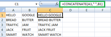
The function merges the data present in the two columns, namely A and B, and displays the result in column C. To get the result for the remaining data, drag the fill handle toward cell C5.

2. Using Ampersand Symbol

In Excel, the ampersand symbol (&) is a text operator that allows you to combine or concatenate two or more text strings into a single cell. It is an alternative to using the CONCATENATE function.

To use the ampersand symbol to concatenate text, you simply need to use the following syntax,

=Text1&Text2&Text3...

Parameters:

Text1, Text2, Text3... are the text strings you want to concatenate.

For example, if you have data in columns A and B and you want to concatenate the data in these columns into column C, you can use the following formula:

=A1&" "&B1

This will concatenate the data in cell A1, followed by a space, and then the data in cell B1 into cell C1.

The ampersand symbol is a quick and easy way to concatenate text strings in Excel, especially when you only need to join two or three. If you need to concatenate more than a few text strings, consider using the CONCATENATE or CONCAT function instead.

Example: Combine the two columns using the ampersand symbol

1. Enter the data in cells A1 and B1.
2. In the column C1 enter the formula as

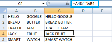
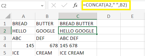
The function merges the data present in the A and B columns and displays the result in column C. To get the result for the remaining data, drag the fill handle toward cell C5.

3. Concat Function

In Excel, the CONCAT function concatenates or joins two or more text strings or cell ranges into a single cell. It is an alternative to using the CONCATENATE function or the "&" operator.

The syntax for the CONCAT function is:

Parameter:

text1, text2, and text3 are the text strings, or cell ranges you want to concatenate.

The square brackets indicate that the argument is optional. Using this function, you can concatenate up to 255 text strings or cell ranges.

For example, if you have data in columns A and B and you want to concatenate the data in these columns into column C, you can use the following formula:

=CONCAT (A1, " ", B1)

This will concatenate the data in cell A1, followed by a space, and then the data in cell B1 into cell C1.

One advantage of the CONCAT function is that it can handle empty cells without displaying error messages. If any arguments are pointless or contain errors, the CONCAT function will ignore them and concatenate the remaining values.

Note: The CONCAT function is available in newer versions of Excel, starting from Excel 2016. If you are using an older version of Excel, you can use the CONCATENATE function or the "&" operator instead.

Example: Combine the two columns of data using the CONCAT function.

1. Enter the data in the column namely A1 and B1.
2. In the cell enter the formula as =CONCAT (A1,"", B1)
3. Press Enter. The CONCAT function combines the selected column of data and displays the result in the selected cell.
   
4. The function merges the data present in the two columns, namely A and B, and displays the result in column C. To get the result for the remaining data, drag the fill handle toward cell C5.

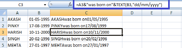
4. How to add additional text with the combined text?

To add additional text to the combined text in Excel, you can include the text in double-quotes within the formula, using the "&" operator.

Here's how to add additional text with the "&" operator:

• Select the cell where you want to combine the columns.
• Type "=" and click on the first cell you want to connect.
• Type "&" and then enclose the additional text in double-quotes.
• Type "&" again, then click on the second cell you want to combine.
• Repeat step 4 for other columns you want to connect.
• Press Enter.

Example: To combine columns A and B and add the text "is a combined text" at the end, you would type =" &A1&" "&B1&" is a combined text" in the cell where you want the combined text to appear.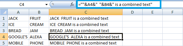

5. Displaying numbers in Combined Cells

To display numbers in combined cells, the steps to be followed are,

1. Enter the data in the worksheet namely A1:B5
2. In cell C1, enter the formula as =A1&"was born on"&TEXT (B1," dd/mm/yyyy").
3. Press Enter.
   
4. The function combines the text in A1 and B1 with the date format.

6. TEXTJOIN Function

TEXTJOIN is a function in Excel that allows you to join text strings from multiple cells into a single cell, separated by a specified delimiter. This function was introduced in Excel 2019 and Excel for Microsoft 365.

Syntax:

The syntax of the TEXTJOIN function is as follows:

Parameter

Delimiter (required): The character or characters to use as a separator between the text strings. This can be any text value, including a space or comma.

ignore_empty (required): A logical value determining whether to ignore empty cells or include them in the result. TRUE ignores empty cells, while FALSE includes them.

text1, [text2]... The text strings join together. You can include up to 252 text arguments.

Here's an example of how to use the TEXTJOIN function in Excel:

Suppose you have a list of names in cells A1:B5, and you want to combine them into a single cell. You could use the following formula:

This formula specifies TRUE for the ignore_empty argument to exclude any empty cells. The range A1:B1 contains the text strings to join.

This formula would result in a single cell with all the names joined together. For example, if the characters in cells A1:B1 were "CHICKEN," "BIRYANI," the result would be "CHICKEN BIRYANI."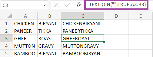

The function merges the data present in the two columns, namely A and B, and displays the result in column C. To get the result for the remaining data, drag the fill handle toward cell C5.

Summary

Merging columns without losing data is a valuable technique that can be used to combine related information from different columns into a single column. This can help to improve data analysis and reduce data redundancy. When merging columns, it is essential to ensure that you keep all necessary information.

To do this, you should carefully consider the data type in each column and how it can be merged. Some standard techniques for joining columns without losing data include concatenation, merging by common identifiers or keys and using pivot tables or other data analysis tools. Overall, merging columns can be a powerful tool for data analysis, but it should be done carefully to ensure that all critical information is retained and correctly accounted for.