Finding Top or Bottom 'N' values in Excel

Microsoft Excel is one of the familiar applications which are used for calculation purposes widely. Excel provides various functions and formulas for calculating the data based on the requirement. Among various functions, one of the functions provided by Excel is to find the top or bottom 'N' values in Excel. Finding the specified 'N' values from the data manually takes time and is difficult. To rectify this problem, Excel provides the necessary formulas to find the specified 'N' values from the given data. The function easily retrieves the specified data from the list. The functions and formulas with examples are explained in this tutorial.

The syntax for Nth largest value

The array is called the first argument of the large function. An absolute reference is provided for the array.

'k' is called the relative reference of the LARGE function. It is used to denote which largest number is required. A relative reference is provided to the number.

The syntax for Nth smallest value

The array is called the first argument of the small function. An absolute reference is provided for the array.

'k' is called the relative reference of the SMALL function. It is used to denote which smallest number is required. A relative reference is provided to the number.

For better understanding, the concept called Cell Reference is explained here.

Cell Reference is sub-divided into the following types,

• Relative Reference
• Absolute Reference

The relative reference and absolute reference concepts are used in the formula to find the top and bottom values in the data.

Relative Reference

• If the formula is dragged down the column, the value will increase
• If the formula is dragged across the row, the alphabet will increase.

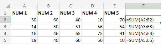
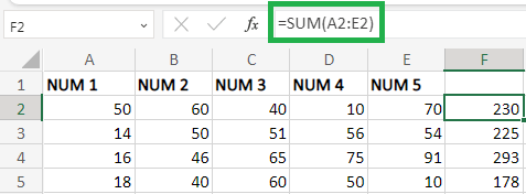
An example for relative reference is explained as follows,

Example 1: Calculate the sum of the given data.

1. Enter the data in the worksheet, namely A1:E5
2. To sum the data which is present in A2:E2, select a new cell, namely F2 and enter the formula as =SUM (A2:E2)
3. The result will be displayed in cell F2. To find the formula for the remaining cells, drag the formula towards F5.
   
   The value in the worksheet will increase while dragging down the formula.
4. Click "Show Formulas" in the formula tab. The formula for the respective cell will display in the column range F2:F5.

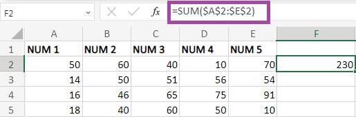
The number increases while the formula is dragged downwards towards the row.

An example for absolute reference is explained as follows,

Example 1.1: Calculate the sum of the given data.

1. Enter the data in the worksheet, namely A1:E5
2. To sum the data which is present in A2:E2, select a new cell namely F2 and enter the formula as =SUM ($A$2:$E$2)
3. The result will be displayed in cell F2.
   
4. Click "Show Formulas" in the formula tab. The formula for the respective cell will display in the column range F2:F5.

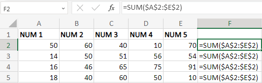
The worksheet's formula remains the same in the column range F2:F5. While going downward in the row, the formula remains the same. This concept is called an absolute reference. It is called an absolute reference.

Example 2: How to find the Top 'N'values from the given list?

To find the top 'N' values from the given data, the steps to be followed are as follows,

1. Enter the data in the worksheet, namely A1:B7
2. Here, in this example, the marks of various students are present in the worksheet. To find the top 3 values from the given data, Select three new cells namely A9, A10, and A11 and type the position number as 1, 2, and 3.
3. In the cell B7 enter the formula as =LARGE ($B$2:$B$7,A9).In the formula B2:B7 is called cell range where the marks are present.A9 denotes the number 'k'.
4. Press Enter. The result will be displayed in cell B7. To get the nth largest value for the other data, drag the formula toward cell A11.

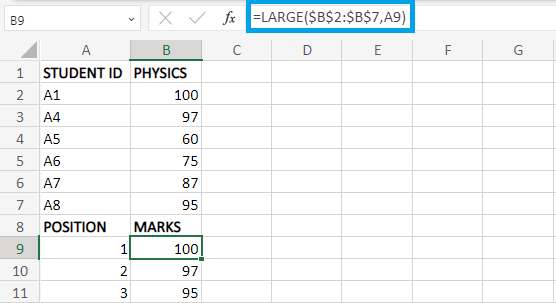
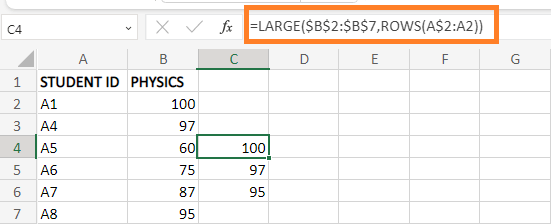
Here in the worksheet, the first, second, and third marks are displayed using the formula. The formula is dragged to the respective cell to find the first three largest numbers.

Example 3: How to find the Bottom 'N'values from the given list?

To find the Bottom 'N' values from the given data, the steps to be followed are as follows,

1. Enter the data in the worksheet, namely A1:B7
2. Here, in this example, the marks of various students are present in the worksheet. To find the bottom 3 values from the given data, Select three new cells, A9, A10, and A11 and type the position number as 1, 2, and 3.
3. In the cell B7 enter the formula as =SMALL ($B$2:$B$7, A9).The formula B2:B7 is called cell range, where the marks are present.A9 denotes the number 'k'.
4. Press Enter. The result will be displayed in cell B7. To get the nth largest value for the other data, drag the formula toward cell A11.

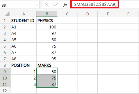
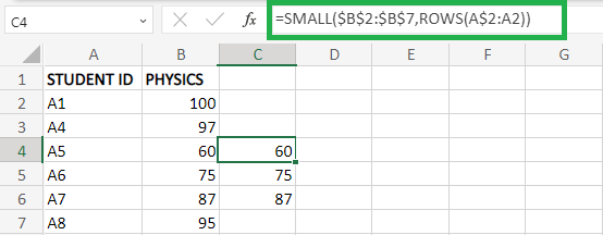
The bottom 'N' values are displayed in the worksheet using the formula. The formula is dragged to the respective cell to find the bottom three values.

Example 4: How to find the Top 'N'values from the given list without mentioning the respective position in the list?

To find the top 'N' values from the given data, without mentioning the necessary position in the list, the steps to be followed are,

1. Enter the data in the worksheet namely A1:B7
2. Here, in this example, the marks of various students are present in the worksheet. To find the top three values from the list, the formula is entered into the new cell
3. In cell C4 enter the formula as =LARGE ($B$2:$B$7, ROWS (A$2: A 2).The formula B2:B7 is called cell range, where the marks are present. A2 represents the column range.
4. Press Enter. The result will be displayed in cell C4. To get the nth largest value for the other data, drag the formula toward cell C6. Here N value is three; hence, to find the first three largest numbers, the formula is dragged toward cell C6.

Examples 1 and 2 mention the position of the 'Nth' value in the worksheet. But in example 3, the nth values are displayed by dragging the formula without mentioning the position of the data.

Example 5: How to find the Bottom 'N'values from the given list without mentioning the respective position in the list?

To find the bottom 'N' values from the given data, without mentioning the necessary position in the list, the steps to be followed are,

1. Enter the data in the worksheet namely A1:B7
2. Here, in this example, the marks of various students are present in the worksheet. To find the bottom three values from the list, the formula is entered into the new cell.
3. In cell C4 enter the formula as =SMALL ($B$2:$B$7, ROWS (A$2: A 2).The formula B2:B7 is called cell range, where the marks are present. A2 represents the column range.
4. Press Enter. The result will be displayed in cell C4. To get the nth bottom value for the other data, drag the formula toward cell C6. Here N value is three; hence, to find the first three bottom numbers, the formula is dragged toward cell C6.

The nth values are displayed by dragging the formula without mentioning the position of the data in the worksheet.

Summary

From the tutorial, the various functions and methods of finding the top or bottom 'N' values are explained briefly. This method helps the user to calculate the data efficiently and quickly.